Day 13 — Stratified Sampling: The Smart Way to Sample

Divide and conquer your sampling strategy for maximum precision.

Stratified sampling guarantees coverage of important subgroups while reducing variance by 50-95% compared to simple random sampling.

Note: This article uses technical terms and abbreviations. For definitions, check out the Key Terms & Glossary page.

The Random Sampling Trap

Imagine you're conducting a health survey in a company of 1,000 employees:

• 900 office workers (90%)

• 100 executives (10%)

You randomly sample 100 people. Here's what can go wrong:

Unlucky Sample #1:

Office workers: 95 people

Executives: 5 people

Problem: Only 5 executives - can't say much about this group!

Unlucky Sample #2:

Office workers: 87 people

Executives: 13 people

Different from reality (90/10 split)!

Unlucky Sample #3:

Office workers: 100 people

Executives: 0 people

Complete miss on executive health!

The problem: Simple Random Sampling (SRS) is... well, random!

The solution: Stratified Sampling - sample smartly within groups!

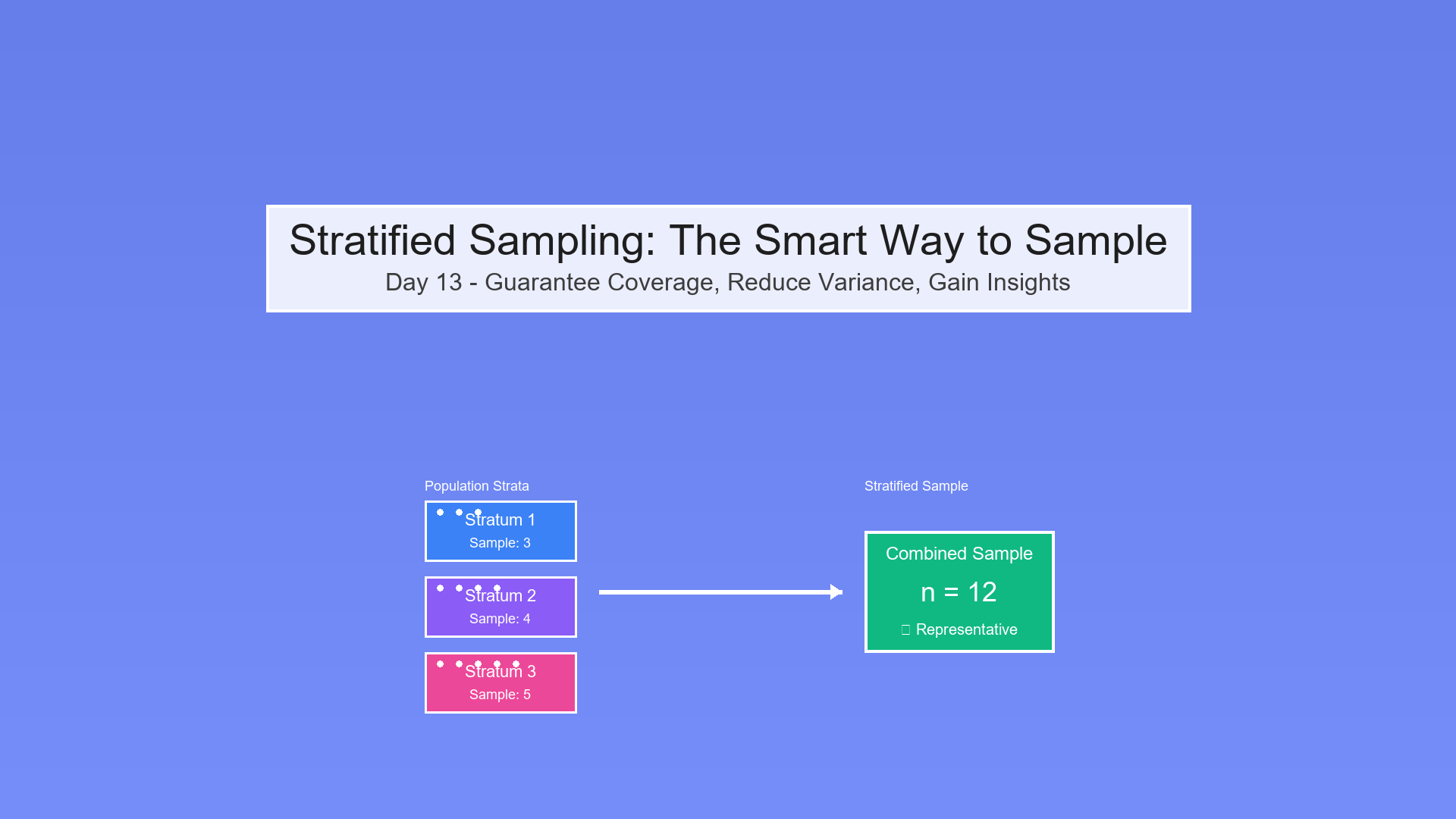
What is Stratified Sampling?

Stratified Sampling means:

1. Divide population into non-overlapping groups (strata)

2. Sample from each stratum separately

3. Combine results with proper weighting

Visual Comparison

Simple Random Sampling (SRS):

Population:  (office workers)

(executive)

Random sample of 10:

Picked:

Result: All office workers!

Stratified Sampling:

Population:

Stratum 1:  (90 office workers)

Stratum 2:  (10 executives)

Stratified sample of 10:

From Stratum 1:  (9 people)

From Stratum 2:  (1 person)

Result: Proper representation!

Why Stratify? Three Big Reasons

1. Guaranteed Coverage

Problem with SRS: Might miss rare but important groups

Example:

City population:

- Urban: 70%

- Suburban: 20%

- Rural: 10%

SRS of 100 might give:

Urban: 65, Suburban: 25, Rural: 10

OR

Urban: 75, Suburban: 22, Rural: 3  ← Rural underrepresented!

Stratified solution:

Explicitly sample from each:

Urban: 70 people (guaranteed)

Suburban: 20 people (guaranteed)

Rural: 10 people (guaranteed)

Coverage ensured!

2. Variance Reduction

The Math Intuition:

Variance comes from differences:

• Between-stratum variance: How different are the groups?

• Within-stratum variance: How different are people within each group?

Key insight: If strata are homogeneous (similar within), stratified sampling has lower variance than SRS!

Visual:

POPULATION (high variance):

Health scores: 45, 48, 50, 52, 85, 87, 88, 90, 91, 92

↑_________↑  ↑___________________↑

Office       Executives

(lower)      (higher)

Within-stratum variance:

Office: σ² = 6.5 (people similar)

Executive: σ² = 7.8 (people similar)

But between-stratum difference is HUGE (50 vs 90)!

SRS estimates affected by this big gap.

Stratified sampling accounts for it separately!

3. Domain Insights

SRS result:

"Average health score: 75"

Okay... but tells us nothing about groups!

Stratified result:

"Average health scores:

Office workers: 52 (95% CI: 50-54)

Executives: 88 (95% CI: 86-90)"

Rich insights about each segment!

The Math: How Much Better Is It?

Variance Formula

Simple Random Sampling variance:

Var(ȳ_SRS) = σ²/n × (N-n)/N

Where:

- σ² = overall population variance

- n = sample size

- N = population size

- (N-n)/N = finite population correction

Stratified Sampling variance:

Var(ȳ_strat) = Σ(Wₕ² × σₕ²/nₕ × (Nₕ-nₕ)/Nₕ)

Where:

- Wₕ = stratum h weight (Nₕ/N)

- σₕ² = variance within stratum h

- nₕ = sample size in stratum h

- Nₕ = population size in stratum h

The Variance Reduction:

Var(ȳ_SRS) - Var(ȳ_strat) = Σ Wₕ(μₕ - μ)²

This is the between-stratum variance!

Translation: The more different your strata are, the bigger the variance reduction!

Example Calculation

Population:

• Stratum 1 (Office): N₁ = 900, μ₁ = 50, σ₁² = 100

• Stratum 2 (Executive): N₂ = 100, μ₂ = 90, σ₂² = 64

• Total: N = 1000

Sample: n = 100

Proportional allocation:

• n₁ = 90 (90% of sample)

• n₂ = 10 (10% of sample)

SRS Variance:

First, calculate overall variance:

μ = 0.9(50) + 0.1(90) = 45 + 9 = 54

σ² = 0.9(100 + (50-54)²) + 0.1(64 + (90-54)²)

= 0.9(100 + 16) + 0.1(64 + 1296)

= 0.9(116) + 0.1(1360)

= 104.4 + 136

= 240.4

Var(ȳ_SRS) = 240.4/100 × (1000-100)/1000

= 2.404 × 0.9

= 2.16

Standard error: √2.16 = 1.47

Stratified Variance:

W₁ = 900/1000 = 0.9

W₂ = 100/1000 = 0.1

Var(ȳ_strat) = 0.9² × (100/90) × (900-90)/900

+ 0.1² × (64/10) × (100-10)/100

= 0.81 × 1.11 × 0.9

+ 0.01 × 6.4 × 0.9

= 0.81 + 0.058

= 0.87

Standard error: √0.87 = 0.93

The Improvement:

Variance reduction: 2.16 - 0.87 = 1.29 (60% reduction! )

Standard error:

SRS: 1.47

Stratified: 0.93

Stratified is 58% more precise!

Translation: To get the same precision with SRS, you'd need 2.5× more samples!

Allocation Strategies: How Many Per Stratum?

Once you decide to stratify, how do you divide your sample across strata?

1. Proportional Allocation (Most Common)

Rule: Sample proportionally to stratum size

nₕ = n × (Nₕ/N)

Example:

Population: 900 office, 100 executive (1000 total)

Sample size: n = 100

Office sample: 100 × (900/1000) = 90

Executive sample: 100 × (100/1000) = 10

Pros:

• Simple, intuitive

• Self-weighting (no complex weights needed)

• Represents population structure

Cons:

• Small strata get small samples (might be imprecise)

2. Equal Allocation 🟰

Rule: Same sample size for each stratum

nₕ = n / H

Where H = number of strata

Example:

Population: 900 office, 100 executive

Sample size: n = 100

Strata: H = 2

Office sample: 100/2 = 50

Executive sample: 100/2 = 50

Pros:

• Good for comparing strata (equal precision)

• Ensures small strata have enough data

Cons:

• Oversamples small strata (need complex weights)

• Less efficient for overall mean estimation

3. Neyman Allocation (Optimal)

Rule: Allocate proportional to stratum size AND variance

nₕ = n × (Nₕ × σₕ) / Σ(Nₖ × σₖ)

Intuition: Sample more from:

• Large strata (more people → more important)

• High-variance strata (more diverse → need more samples)

Example:

Stratum 1: N₁ = 900, σ₁ = 10

Stratum 2: N₂ = 100, σ₂ = 8

Stratum 1 weight: 900 × 10 = 9,000

Stratum 2 weight: 100 × 8 = 800

Total weight: 9,800

Office sample: 100 × (9000/9800) = 91.8 ≈ 92

Executive sample: 100 × (800/9800) = 8.2 ≈ 8

Pros:

• Mathematically optimal (minimizes variance!)

• Accounts for both size and heterogeneity

Cons:

• Requires knowing σₕ in advance (often unknown!)

• Might still undersample important small strata

4. Optimal Allocation with Cost

Rule: Account for different sampling costs per stratum

nₕ = n × (Nₕ × σₕ / √cₕ) / Σ(Nₖ × σₖ / √cₖ)

Where cₕ = cost to sample one unit from stratum h

Example:

Executives cost 5× more to survey (busy, need incentives)

c₁ = $10 (office worker)

c₂ = $50 (executive)

This would reduce executive sample further!

Use when: Budget constrained, different costs per stratum

Visual: Variance vs Allocation

Let's see how variance changes with different allocations:

Variance (SE²)

3.0

•  SRS

2.5

2.0          • Equal

1.5

1.0                 • Proportional

0.5                          • Neyman

(Optimal!)

0.0

Different Allocation Strategies

Lower is better!

Takeaway: Neyman always wins (if you know the variances)!

Defining Strata: The Art and Science

Good strata are:

1. Mutually Exclusive

Each unit belongs to exactly one stratum

Bad: "Young", "Students"

(Young students counted twice!)

Good: "Student", "Non-Student"

2. Exhaustive

Every unit belongs to some stratum

Bad: "<30", "40-60", ">60"

(Missing 30-40 age range!)

Good: "<30", "30-40", "40-60", ">60"

3. Homogeneous Within 🟰

Units within stratum are similar

Bad stratum: "People" (too diverse!)

Good stratum: "Female doctors aged 40-50"

4. Heterogeneous Between

Strata are different from each other

Bad: "Age 30-40", "Age 31-41"

(Too much overlap, not distinct!)

Good: "Age 18-30", "Age 31-50", "Age 51+"

5. Meaningful

Based on domain knowledge, not arbitrary

Bad: "First 500 rows", "Last 500 rows"

(Arbitrary split!)

Good: "Urban", "Suburban", "Rural"

(Meaningful demographic divisions)

Common Stratification Variables:

Demographics:

• Age groups

• Gender

• Education level

• Income brackets

• Geographic region

Business:

• Customer segments (high/medium/low value)

• Product categories

• Time periods (Q1, Q2, Q3, Q4)

Medical:

• Disease severity (mild/moderate/severe)

• Treatment type

• Risk factors present/absent

Exercise: SRS vs Stratified Variance

Let's work through a complete example!

The Setup

Population of 20 people:

Stratum 1 (Group A) - 15 people:

Values: [10, 11, 12, 13, 14, 15, 16, 17, 18, 19, 20, 21, 22, 23, 24]

Mean (μ₁) = 17

Variance (σ₁²) = 20

SD (σ₁) = 4.47

Stratum 2 (Group B) - 5 people:

Values: [50, 52, 54, 56, 58]

Mean (μ₂) = 54

Variance (σ₂²) = 8

SD (σ₂) = 2.83

Overall population:

N = 20

μ = (15×17 + 5×54)/20 = (255 + 270)/20 = 26.25

We want to sample n = 8 people.

Approach 1: Simple Random Sampling

Variance calculation:

First, overall variance:

σ² = Σ(xᵢ - μ)² / N

For stratum 1 contribution:

= (15/20) × [σ₁² + (μ₁ - μ)²]

= 0.75 × [20 + (17 - 26.25)²]

= 0.75 × [20 + 85.56]

= 0.75 × 105.56

= 79.17

For stratum 2 contribution:

= (5/20) × [σ₂² + (μ₂ - μ)²]

= 0.25 × [8 + (54 - 26.25)²]

= 0.25 × [8 + 770.06]

= 0.25 × 778.06

= 194.52

Total: σ² = 79.17 + 194.52 = 273.69

Var(ȳ_SRS) = σ²/n × (N-n)/N

= 273.69/8 × (20-8)/20

= 34.21 × 0.6

= 20.53

Standard Error: √20.53 = 4.53

Approach 2: Proportional Stratified Sampling

Sample allocation:

n₁ = 8 × (15/20) = 6

n₂ = 8 × (5/20) = 2

Variance calculation:

W₁ = 15/20 = 0.75

W₂ = 5/20 = 0.25

Var(ȳ_strat) = W₁² × (σ₁²/n₁) × (N₁-n₁)/N₁

+ W₂² × (σ₂²/n₂) × (N₂-n₂)/N₂

= 0.75² × (20/6) × (15-6)/15

+ 0.25² × (8/2) × (5-2)/5

= 0.5625 × 3.33 × 0.6

+ 0.0625 × 4 × 0.6

= 1.125 + 0.15

= 1.275

Standard Error: √1.275 = 1.13

Approach 3: Neyman Allocation

Optimal allocation:

Stratum 1: N₁ × σ₁ = 15 × 4.47 = 67.05

Stratum 2: N₂ × σ₂ = 5 × 2.83 = 14.15

Total: 81.20

n₁ = 8 × (67.05/81.20) = 6.6 ≈ 7

n₂ = 8 × (14.15/81.20) = 1.4 ≈ 1

Variance calculation:

Var(ȳ_Neyman) = 0.75² × (20/7) × 0.53

+ 0.25² × (8/1) × 0.8

= 0.5625 × 2.86 × 0.53

+ 0.0625 × 8 × 0.8

= 0.85 + 0.40

= 1.25

Standard Error: √1.25 = 1.12

The Comparison Table

| Method | n₁ | n₂ | Variance | SE | Efficiency |

|--------|----|----|----------|-----|------------|

| SRS | varies | varies | 20.53 | 4.53 | 1.00× |

| Proportional | 6 | 2 | 1.275 | 1.13 | 16.1× |

| Neyman | 7 | 1 | 1.25 | 1.12 | 16.4× |

Key Insights:

Stratified sampling reduces variance by 94%! (From 20.53 to 1.27)

Why? The two groups are VERY different (means of 17 vs 54), but within each group, people are similar

Neyman only slightly better than proportional (1.25 vs 1.275) - proportional is good enough!

To match stratified precision with SRS, you'd need 129 samples instead of 8! (16× more)

Visual Representation

Standard Error Comparison

SRS:          (4.53)

Proportional:  (1.13)

Neyman:        (1.12)

Shorter bars = Better (more precise)!

Python Implementation

perform_stratification Function

import pandas as pd
import numpy as np

def perform_stratification(df, stratum_col, target_col,
sample_size, allocation='proportional'):
"""
Perform stratified sampling

Parameters:
- df: DataFrame
- stratum_col: Column defining strata
- target_col: Variable of interest
- sample_size: Total sample size
- allocation: 'proportional', 'equal', or 'neyman'

Returns:
- sample_df: Stratified sample
- summary: Allocation summary
"""

# Calculate stratum statistics
stratum_stats = df.groupby(stratum_col).agg({
target_col: ['count', 'mean', 'std']
}).reset_index()

stratum_stats.columns = [stratum_col, 'N', 'mean', 'std']
stratum_stats['weight'] = stratum_stats['N'] / len(df)

# Calculate sample sizes per stratum
if allocation == 'proportional':
stratum_stats['n'] = (
sample_size * stratum_stats['weight']
).round().astype(int)

elif allocation == 'equal':
n_strata = len(stratum_stats)
stratum_stats['n'] = sample_size // n_strata

elif allocation == 'neyman':
# Optimal allocation
stratum_stats['allocation_weight'] = (
stratum_stats['N'] * stratum_stats['std']
)
total_weight = stratum_stats['allocation_weight'].sum()
stratum_stats['n'] = (
sample_size * stratum_stats['allocation_weight'] / total_weight
).round().astype(int)

# Adjust for rounding errors
total_allocated = stratum_stats['n'].sum()
if total_allocated != sample_size:
diff = sample_size - total_allocated
# Add/subtract from largest stratum
largest_idx = stratum_stats['N'].idxmax()
stratum_stats.loc[largest_idx, 'n'] += diff

# Perform stratified sampling
sample_dfs = []
for _, row in stratum_stats.iterrows():
stratum_data = df[df[stratum_col] == row[stratum_col]]
stratum_sample = stratum_data.sample(
n=int(row['n']),
replace=False,
random_state=42
)
sample_dfs.append(stratum_sample)

sample_df = pd.concat(sample_dfs, ignore_index=True)

return sample_df, stratum_stats

def show_stratification_summary(stratum_stats, allocation_type):
"""
Display stratification summary with variance estimates
"""
print(f"\n{'='*60}")
print(f"Stratification Summary - {allocation_type.title()} Allocation")
print(f"{'='*60}\n")

print(stratum_stats.to_string(index=False))

# Calculate overall variance
total_n = stratum_stats['n'].sum()

variance_components = (
stratum_stats['weight']**2 *
stratum_stats['std']**2 / stratum_stats['n'] *
(stratum_stats['N'] - stratum_stats['n']) / stratum_stats['N']
)

total_variance = variance_components.sum()
se = np.sqrt(total_variance)

print(f"\n{'='*60}")
print(f"Overall Variance: {total_variance:.4f}")
print(f"Standard Error: {se:.4f}")
print(f"{'='*60}\n")

return total_variance, se

Usage Example

# Create toy dataset
np.random.seed(42)
df = pd.DataFrame({
'group': ['A']*150 + ['B']*50,
'value': np.concatenate([
np.random.normal(50, 10, 150),  # Group A
np.random.normal(90, 8, 50)     # Group B
])
})

# Proportional allocation
sample_prop, stats_prop = perform_stratification(
df, 'group', 'value',
sample_size=100,
allocation='proportional'
)
var_prop, se_prop = show_stratification_summary(stats_prop, 'proportional')

# Neyman allocation
sample_neyman, stats_neyman = perform_stratification(
df, 'group', 'value',
sample_size=100,
allocation='neyman'
)
var_neyman, se_neyman = show_stratification_summary(stats_neyman, 'neyman')

# Compare with SRS
overall_std = df['value'].std()
var_srs = overall_std**2 / 100 * (200-100)/200
se_srs = np.sqrt(var_srs)

print(f"\nComparison:")
print(f"SRS SE: {se_srs:.4f}")
print(f"Proportional SE: {se_prop:.4f} ({(1-se_prop/se_srs)*100:.1f}% reduction)")
print(f"Neyman SE: {se_neyman:.4f} ({(1-se_neyman/se_srs)*100:.1f}% reduction)")

When to Use Stratified Sampling

Perfect For:

Known subgroups that differ meaningfully

• Demographics (age, gender, region)

• Business segments (customer tiers)

• Risk categories (low/medium/high)

Small important groups you must include

• Rare diseases

• Executive opinions

• Minority populations

Variance reduction is critical

• Limited budget (need maximum precision)

• Policy decisions (small errors matter)

• Clinical trials (safety critical)

Domain insights needed per group

• Compare regions

• Track segments over time

• Identify disparities

Don't Use When:

No clear strata exist

• Homogeneous population

• Unknown groupings

• Exploratory research (don't know what matters)

Stratum information unavailable at sampling time

• Can't identify strata before sampling

• Post-hoc stratification (use weighting instead)

Very small sample sizes

• n < 30: Stratification overhead not worth it

• Not enough samples per stratum

Cost prohibitive

• Different strata require vastly different effort

• Geographic dispersion makes stratified sampling impractical

Common Pitfalls

1. Too Many Strata

Bad: 20 strata with n=100 samples

→ 5 samples per stratum (unreliable!)

Good: 4-5 strata with n=100 samples

→ 20-25 per stratum (stable estimates)

Rule of thumb: At least 10-15 samples per stratum

2. Ignoring Weights

With non-proportional allocation, you MUST weight results:

# Wrong (unweighted)
overall_mean = sample_df['value'].mean()

# Right (weighted)
stratum_means = sample_df.groupby('stratum')['value'].mean()
stratum_weights = population_stratum_sizes / population_total
overall_mean = (stratum_means * stratum_weights).sum()

3. Defining Overlapping Strata

Bad:

Stratum A: "Students"

Stratum B: "Age < 25"

→ Young students belong to both!

Good:

Stratum A: "Student, Age < 25"

Stratum B: "Student, Age ≥ 25"

Stratum C: "Non-student, Age < 25"

Stratum D: "Non-student, Age ≥ 25"

4. Forgetting Finite Population Correction

When sampling a large fraction of the stratum:

# Include FPC
var_stratum = (sigma²/n) * (N-n)/N

# Not just
var_stratum = sigma²/n  # Wrong!

Takeaway

Stratified sampling is the "divide and conquer" of sampling:

Key Concepts:

Strata = non-overlapping, exhaustive groups

Proportional allocation = sample proportionally (simple, self-weighting)

Neyman allocation = optimal (proportional to Nₕ × σₕ)

Variance reduction = can be 50-95% lower than SRS!

Coverage guarantee = ensures rare groups included

Domain insights = separate estimates per stratum

The Math Win:

Variance reduction = Σ Wₕ(μₕ - μ)²

Translation: The more different your strata,

the bigger the improvement!

Allocation Decision Tree:

Do you know σₕ for each stratum?

Yes → Use Neyman (optimal!)

No → Do you need equal precision per stratum?

Yes → Use Equal allocation

No → Use Proportional (simplest)

Real Impact:

In our exercise, stratified sampling gave 16× more precision than SRS with the same sample size. That's like getting 129 samples for the price of 8!

References

1. Cochran, W. G. (1977). Sampling Techniques (3rd ed.). John Wiley & Sons.

2. Lohr, S. L. (2019). Sampling: Design and Analysis (3rd ed.). Chapman and Hall/CRC.

3. Kish, L. (1965). Survey Sampling. John Wiley & Sons.

4. Neyman, J. (1934). On the two different aspects of the representative method: The method of stratified sampling and the method of purposive selection. Journal of the Royal Statistical Society, 97(4), 558-625.

5. Särndal, C. E., Swensson, B., & Wretman, J. (1992). Model Assisted Survey Sampling. Springer-Verlag.

6. Thompson, S. K. (2012). Sampling (3rd ed.). John Wiley & Sons.

7. Valliant, R., Dever, J. A., & Kreuter, F. (2018). Practical Tools for Designing and Weighting Survey Samples (2nd ed.). Springer.

8. Groves, R. M., Fowler, F. J., Couper, M. P., Lepkowski, J. M., Singer, E., & Tourangeau, R. (2009). Survey Methodology (2nd ed.). John Wiley & Sons.

9. Little, R. J., & Rubin, D. B. (2019). Statistical Analysis with Missing Data (3rd ed.). John Wiley & Sons.

10. Lumley, T. (2010). Complex Surveys: A Guide to Analysis Using R. John Wiley & Sons.

Note: This article uses technical terms like stratified sampling, variance reduction, allocation, Neyman allocation, and finite population correction. For definitions, check out the Key Terms & Glossary page.