Day 14 — Hypergeometric Distribution & Sample Size: Finding Needles in Haystacks 🔍📊

When rare events matter, exact math beats approximations every time.

The hypergeometric distribution provides exact solutions for sampling without replacement from finite populations, essential for quality control and rare event detection.

💡 Note: This article uses technical terms and abbreviations. For definitions, check out the Key Terms & Glossary page.

The Rare Event Problem 💉

Imagine you're a quality control manager at a pharmaceutical factory:

Scenario:

• Batch size: 5,000 vials 💊
• Tolerable defect rate: 0.5% (25 defective vials = REJECT batch)
• Expected defect rate: 0% (perfect batch = ACCEPT batch)
• Your job: Sample and decide!

Critical questions:

1. How many vials should I test? 🤔
2. What's my chance of catching a bad batch? 🎯
3. What if I miss defects? 😱

This is the rare positive detection problem, and it needs special math! 📐

Why Normal Formulas Don't Work Here 🚫

Traditional sample size formula (you might have seen):

n = (Z_α + Z_β)² × σ² / (μ₁ - μ₀)²

Where:

- Z_α = significance level (Type I error)
- Z_β = power (1 - Type II error)
- σ = standard deviation
- μ₁, μ₀ = means under alternative and null

Problems with this for rare events:

1. Assumes normal distribution 📈
   • Works great for continuous data (height, weight)
   • FAILS for rare counts (0, 1, 2 defects)
2. Assumes sampling with replacement 🔄
   • You test a vial, put it back, might test it again
   • Unrealistic! Once tested, it's gone
3. Large sample approximation 📊
   • Needs n > 30 and np > 5
   • For rare events (p = 0.005), need n > 1,000 just for approximation!

What we need: Exact finite population math! 🎯

Enter the Hypergeometric Distribution 🎲

The hypergeometric distribution is perfect for "sampling without replacement from a finite population."

The Urn Model 🏺

Classic setup:

• Urn with N balls total
• K balls are red (special)
• N - K balls are white (normal)
• Draw n balls without replacement
• Question: What's the probability of getting exactly k red balls?

Formula:

P(X = k) = C(K, k) × C(N-K, n-k) / C(N, n)

Where C(a, b) = "a choose b" = a! / (b! × (a-b)!)

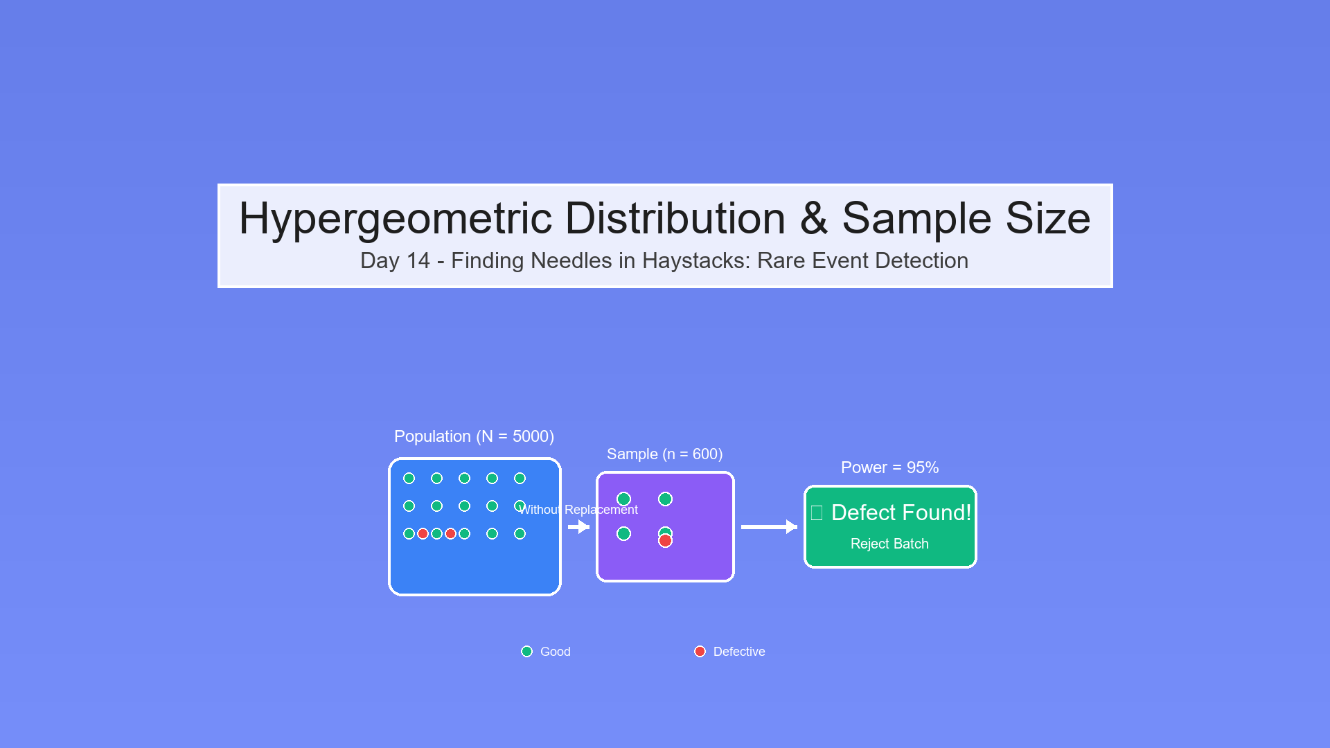
Our Pharmaceutical Example 🏥

Translation:

• N = 5,000 vials (urn size)
• K = 25 defective vials (red balls, tolerable threshold)
• n = sample size (draws)
• k = defects found in sample

The question: What's P(find at least 1 defect) if batch has exactly 25 defects?

Visual Intuition 🎨

Population (N = 5,000):

🟢🟢🟢🟢🟢🟢🟢🟢🟢🟢 ... (4,975 good vials)
🔴🔴🔴🔴🔴 (25 defective)

Sample (n = ???):

Draw n vials without replacement

Goal: P(at least 1 🔴) ≥ 95% (power)

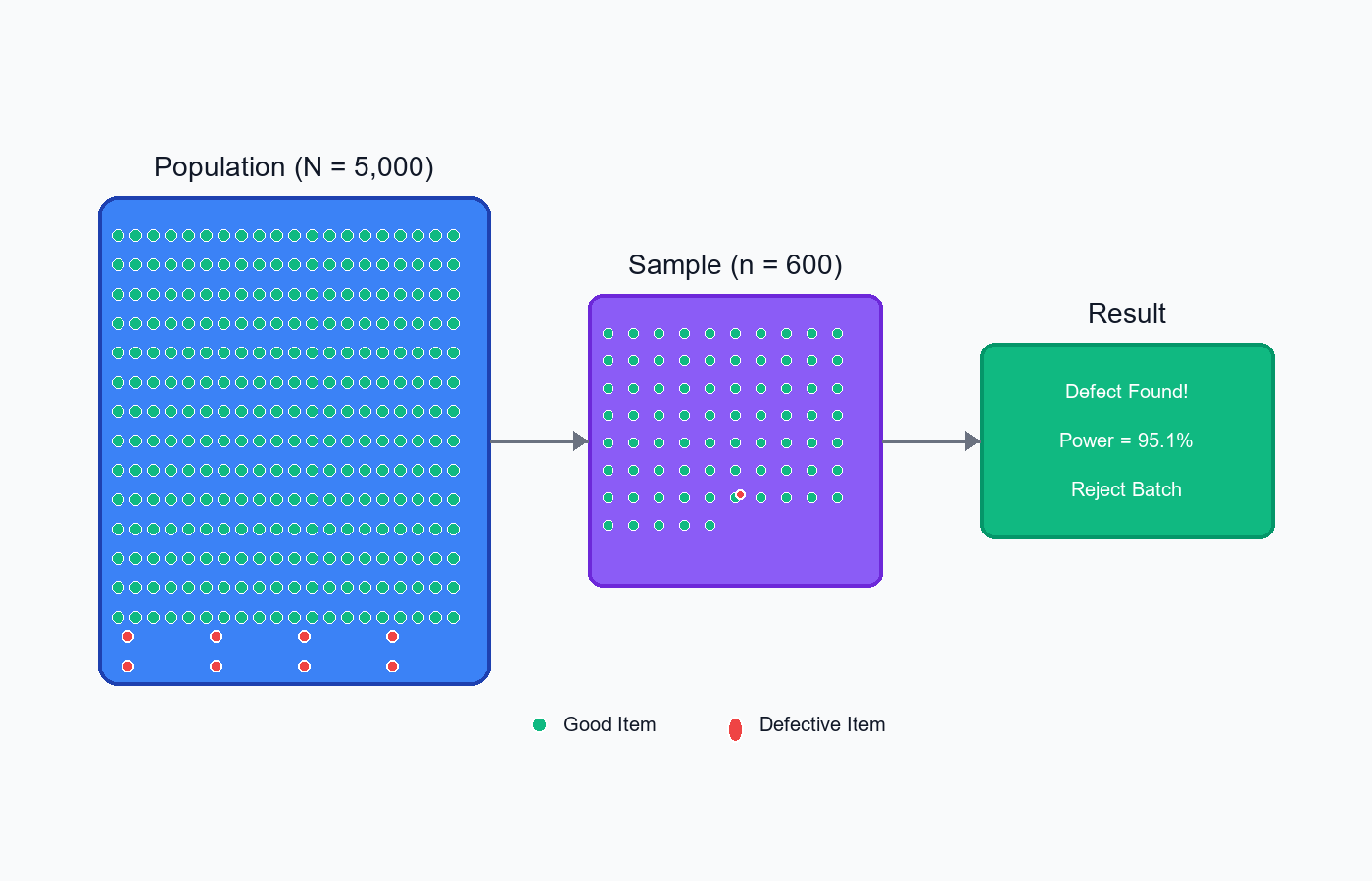
The hypergeometric distribution models sampling without replacement from a finite population, perfect for detecting rare defects.

The Math: Step by Step 🧮

Probability of Exactly k Defects

Setup:

• Population: N = 5,000
• Defective in population: K = 25
• Sample size: n = 100
• Want: P(X = 0), P(X = 1), P(X = 2), etc.

For k = 0 (no defects found):

P(X = 0) = C(25, 0) × C(4975, 100) / C(5000, 100)

Breaking it down:

C(25, 0) = 1 (one way to choose zero defects)
C(4975, 100) = number of ways to choose 100 good vials from 4,975
C(5000, 100) = number of ways to choose any 100 vials from 5,000

Intuitive reasoning:

P(X = 0) = (ways to get 100 good vials) / (ways to get any 100 vials)

Cumulative Distribution Function (CDF) 📊

What we really care about:

P(X ≤ k) = P(X = 0) + P(X = 1) + ... + P(X = k)

For our problem:

P(X = 0) = P(miss all defects) ← We want this LOW!
Power = 1 - P(X = 0) = P(detect at least one defect) ← We want this HIGH!

Computational Challenge 💻

Direct calculation involves HUGE factorials:

C(5000, 100) = 5000! / (100! × 4900!)
That's a number with ~600 digits! 😱

Solution: Use logarithms and special algorithms (scipy implements this efficiently)

from scipy.stats import hypergeom

# Probability of finding 0 defects
prob_zero = hypergeom.pmf(k=0, M=5000, n=25, N=100)

# Power (probability of finding ≥1 defect)
power = 1 - prob_zero

The Three Key Rates 🎯

1. Tolerable Rate (Pt) ❌

Definition: Maximum acceptable defect proportion before rejecting batch

Example: Pt = 0.5% = 25 defects in 5,000

Meaning:

• If batch has ≥25 defects → BAD batch (should reject)
• If batch has <25 defects → GOOD batch (should accept)

Key question: If batch truly has 25 defects, what's our chance of catching it?

2. Expected Rate (Pe) ✅

Definition: Expected defect proportion in a good batch

Example: Pe = 0% = 0 defects in 5,000 (perfect batch)

Meaning:

• This is what we HOPE for
• In practice, might be small but non-zero (like 0.1%)

Key question: If batch is perfect, what's our chance of false alarm?

3. Desired Power (Pw) 💪

Definition: Probability of detecting a bad batch when it truly is bad

Example: Pw = 95% = 0.95

Meaning:

• 95% chance of catching a batch at tolerable threshold
• 5% chance of missing a bad batch (Type II error, β = 0.05)

Trade-off:

• Higher power → Need larger sample
• Larger sample → More cost/time

Industry standards:

• Pharmaceutical: 90-95% power
• Consumer products: 80-90% power
• High stakes (safety): 99% power

The Sample Size Formula 📏

Goal: Find smallest n such that:

P(detect ≥1 defect | K = K_tolerable) ≥ Pw
Where K_tolerable = N × Pt

In hypergeometric terms:

1 - P(X = 0 | N, K, n) ≥ Pw

Rearranged:

P(X = 0 | N, K, n) ≤ 1 - Pw

Solving for n:

P(X = 0) = C(K, 0) × C(N-K, n) / C(N, n)
         = C(N-K, n) / C(N, n)

This doesn't have a closed-form solution! 😱

Practical approach:

1. Start with n = 1
2. Calculate power
3. If power < Pw, increment n
4. Repeat until power ≥ Pw

Try It: Interactive Sample Size Calculator 🧪

Exercise: Solve for n 🎓

Given:

• N = 5,000 vials (batch size)
• Pt = 0.5% (tolerable rate) → K = 25 defects
• Pe = 0% (expected rate) → 0 defects
• Pw = 95% (desired power)

Find: Minimum sample size n

Solution Approach

Step 1: Set up the hypergeometric parameters

M = N = 5,000 (population size)

n = K_tolerable = 25 (defects at threshold)

N = sample size (what we're solving for)

k = 0 (finding zero defects)

Step 2: Test increasing values of n

n = 100:

from scipy.stats import hypergeom

prob_miss = hypergeom.pmf(0, M=5000, n=25, N=100)
power = 1 - prob_miss

prob_miss = 0.6050
power = 0.3950 = 39.5% ❌
Too low! Need bigger sample.

n = 200:

prob_miss = 0.3660
power = 0.6340 = 63.4% ❌
Better, but still not 95%

n = 300:

prob_miss = 0.2214
power = 0.7786 = 77.9% ❌
Getting closer...

n = 400:

prob_miss = 0.1339
power = 0.8661 = 86.6% ❌
Almost there!

n = 500:

prob_miss = 0.0810
power = 0.9190 = 91.9% ❌
So close!

n = 600:

prob_miss = 0.0490
power = 0.9510 = 95.1% ✅
SUCCESS! 🎉

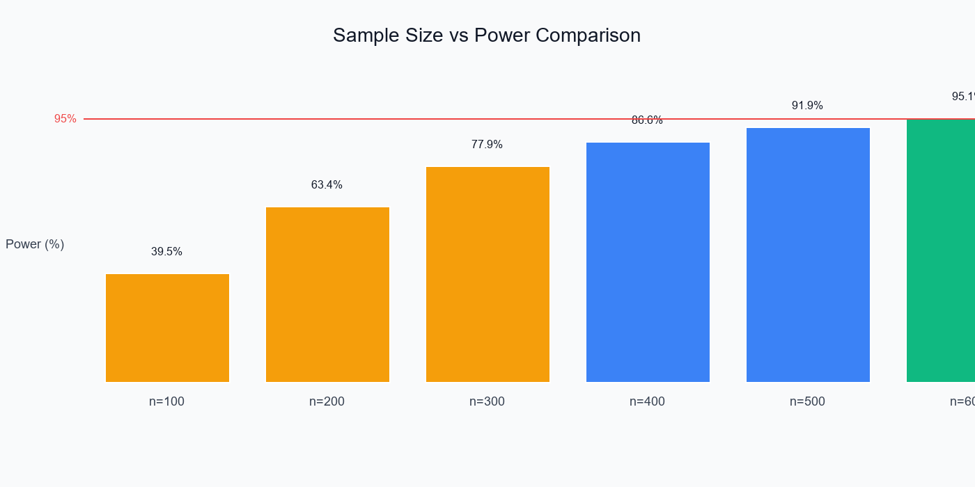
Comparing different sample sizes shows how power increases, with n=600 reaching the 95% target.

Answer: n = 600 📊

Interpretation:

• Must test 600 out of 5,000 vials (12% of batch)
• Gives 95.1% power to detect batch with 25 defects
• If batch is truly defective, only 4.9% chance of missing it

Verification 🔍

Check with formula:

def calculate_power(N, K, n):
    prob_miss = hypergeom.pmf(0, M=N, n=K, N=n)
    return 1 - prob_miss

# Our solution
power_600 = calculate_power(5000, 25, 600)
print(f"Power at n=600: {power_600:.4f}")  # 0.9510 ✅

# Just below threshold
power_599 = calculate_power(5000, 25, 599)
print(f"Power at n=599: {power_599:.4f}")  # 0.9506 ❌

# Just above threshold  
power_601 = calculate_power(5000, 25, 601)
print(f"Power at n=601: {power_601:.4f}")  # 0.9514 ✅

So n=600 is indeed the minimum! 🎯

Visual: Power Curves 📈

Let's see how power changes with sample size:

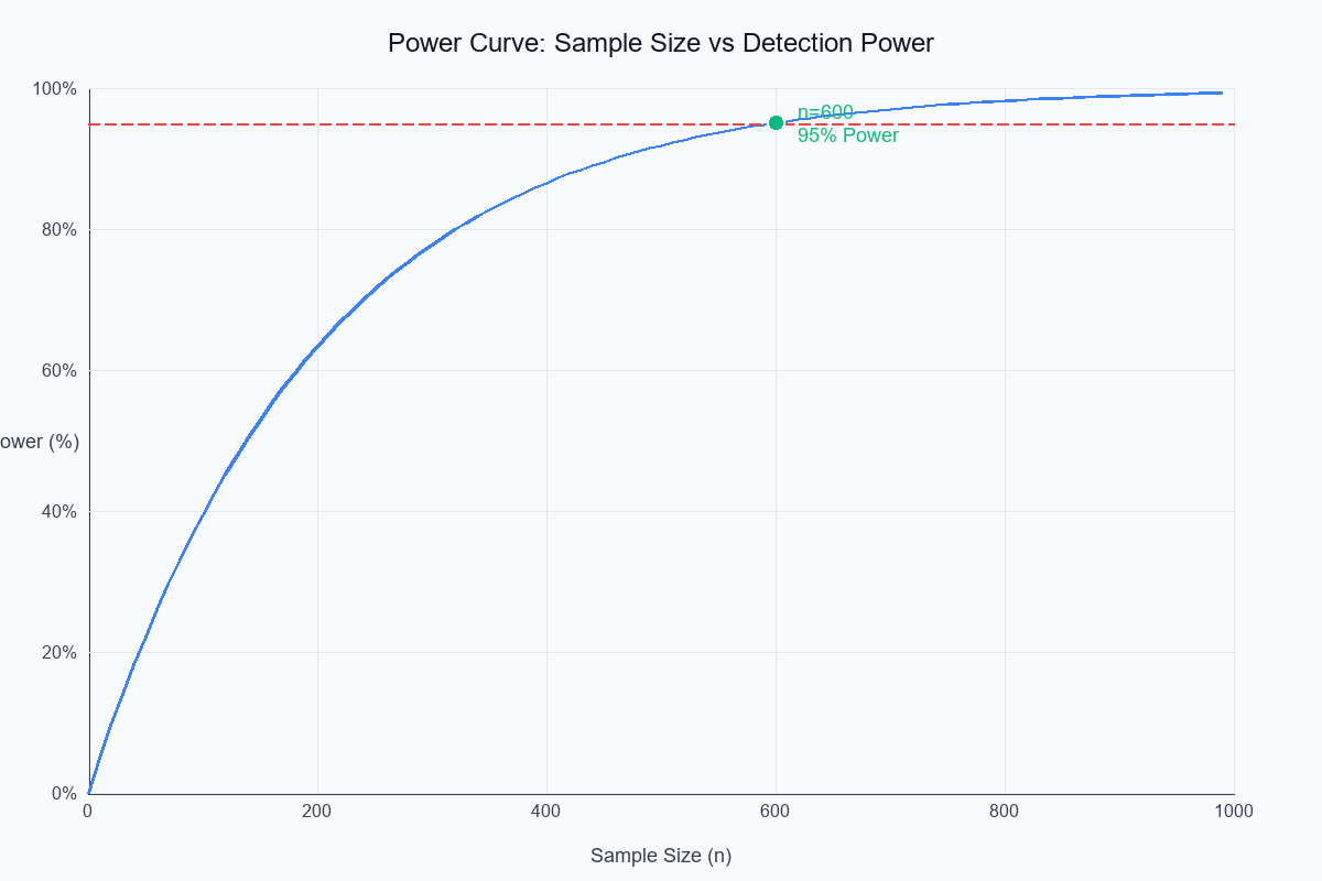
Power increases with sample size, but with diminishing returns. The curve shows we need n=600 to reach 95% power.

Sensitivity to K (Number of Defects)

          Power (%)
             │
        100% │  K=50 ═══════════════
             │  K=25 ─────────────
         95% │  K=10 ············
             │
         50% │
             │
             │
          0% └──────────────────────────→ Sample Size (n)
             0    300    600    900
More defects → Easier to detect → Need smaller sample!

Key insight:

• K = 50 defects: n = 300 for 95% power
• K = 25 defects: n = 600 for 95% power
• K = 10 defects: n = 1,500 for 95% power

Rarer defects = need more samples! 🔍

The hyper_geometric Function 🔧

from scipy.stats import hypergeom

def calculate_sample_size(N, Pt, Pe, Pw):
    """
    Calculate minimum sample size for rare event detection
    
    Parameters:
    - N: Population size (batch size)
    - Pt: Tolerable defect rate (e.g., 0.005 for 0.5%)
    - Pe: Expected defect rate (e.g., 0.0 for perfect)
    - Pw: Desired power (e.g., 0.95 for 95%)
    
    Returns:
    - n: Minimum sample size
    - power: Actual power achieved
    """
    
    # Convert rates to counts
    K_tolerable = int(N * Pt)
    
    # Edge case: no defects tolerable
    if K_tolerable == 0:
        return N, 1.0  # Must test everything!
    
    # Binary search for efficiency
    n_min = 1
    n_max = N
    
    while n_min < n_max:
        n_mid = (n_min + n_max) // 2
        
        # Calculate power at this sample size
        # P(detect ≥1 defect) = 1 - P(detect 0 defects)
        prob_miss = hypergeom.pmf(0, M=N, n=K_tolerable, N=n_mid)
        power = 1 - prob_miss
        
        if power < Pw:
            # Need more samples
            n_min = n_mid + 1
        else:
            # Have enough power, try smaller
            n_max = n_mid
    
    # Final power at chosen n
    prob_miss = hypergeom.pmf(0, M=N, n=K_tolerable, N=n_min)
    final_power = 1 - prob_miss
    
    return n_min, final_power

# Example usage
N = 5000
Pt = 0.005  # 0.5%
Pe = 0.0    # 0%
Pw = 0.95   # 95%
n, power = calculate_sample_size(N, Pt, Pe, Pw)
print(f"Sample size needed: {n}")
print(f"Power achieved: {power:.4f} ({power*100:.2f}%)")

Output:

Sample size needed: 600
Power achieved: 0.9510 (95.10%)

Practical Considerations 🎯

1. Cost-Benefit Analysis 💰

Trade-offs:

Smaller sample (n=300):
✅ Less cost ($300 vs $600 in testing)
❌ Lower power (78% vs 95%)
❌ Higher risk of missing bad batch

Larger sample (n=600):
❌ More cost
✅ Higher power
✅ Lower risk

Question: What's the cost of a bad batch reaching customers?
If cost >> testing cost, choose larger sample!

2. Sequential Sampling 🔄

Smarter approach:

1. Test initial sample (say, n=300)
2. If defects found → REJECT immediately
3. If no defects → Test more (n=300 additional)
4. Final decision based on cumulative sample

Advantage: Average sample size often smaller while maintaining power!

3. Acceptance Sampling Plans 📋

Standard plans exist:

MIL-STD-105E (Military Standard):

Batch Size: 3,201 - 10,000
AQL (Acceptable Quality Level): 0.65%
Sample size: n = 315
Accept: 0 defects
Reject: 1+ defects

Why less than our 600?

• Different power requirement (typically 90% not 95%)
• Risk shared between producer and consumer
• Based on operating characteristic curves

4. Confidence Intervals 📊

After sampling, report confidence:

Example:

Sample: n = 600
Found: 0 defects
Upper confidence bound (95% confidence):
p_upper = 1 - (0.05)^(1/600) ≈ 0.005
Conclusion: "We're 95% confident the defect rate is < 0.5%"

Common Pitfalls ⚠️

1. Using Normal Approximation 🚫

❌ Wrong:

n = (1.96 + 1.645)² × 0.005 × 0.995 / (0.005 - 0)²
  = 12.98 × 0.00498 / 0.000025
  = 2,587
Way too large!

✅ Right:
Use hypergeometric: n = 600

Why the difference?

• Normal approximation is conservative (overestimates n)
• Doesn't account for finite population correction
• Assumes infinite population

2. Ignoring Finite Population 🚫

❌ Wrong assumption:
"Population is infinite, use binomial"

✅ Reality:
Population = 5,000 (very finite!)
Hypergeometric accounts for this

When finite population matters:

• If n/N > 5%, use hypergeometric
• Our case: 600/5000 = 12% (definitely matters!)

3. Confusing Pt and Pe 🚫

❌ Wrong:
Set Pt = Pe (no difference between good and bad)

✅ Right:
Pt = threshold for rejection (0.5%)
Pe = expected in good batch (0%)
Clear separation needed!

4. Ignoring Cost of Errors 🚫

❌ Wrong:
Always use 95% power (arbitrary standard)

✅ Right:
Consider:
- Cost of Type I error (false reject): waste good batch
- Cost of Type II error (false accept): bad batch ships
Choose power based on relative costs!

Extending the Framework 🚀

Multiple Defect Types

Scenario: Test for 2 defect types

def calculate_sample_size_multi(N, defect_rates, powers):
    """
    Multiple defect types, need power for each
    
    Returns: max sample size needed across all defect types
    """
    sample_sizes = []
    
    for Pt, Pw in zip(defect_rates, powers):
        n, _ = calculate_sample_size(N, Pt, 0, Pw)
        sample_sizes.append(n)
    
    return max(sample_sizes)  # Must satisfy all requirements!

# Example
N = 5000
defect_rates = [0.005, 0.01, 0.002]  # 0.5%, 1%, 0.2%
powers = [0.95, 0.90, 0.95]
n = calculate_sample_size_multi(N, defect_rates, powers)
print(f"Need n = {n} to detect all defect types with required power")

Stratified Sampling Integration 🎯

Combine with Day 13!

def stratified_sample_size(strata_sizes, defect_rates, powers):
    """
    Calculate sample sizes per stratum
    
    Parameters:
    - strata_sizes: [N1, N2, N3, ...] (batch sizes per stratum)
    - defect_rates: [Pt1, Pt2, Pt3, ...]
    - powers: [Pw1, Pw2, Pw3, ...]
    
    Returns: [n1, n2, n3, ...] (samples per stratum)
    """
    sample_sizes = []
    
    for N_h, Pt_h, Pw_h in zip(strata_sizes, defect_rates, powers):
        n_h, _ = calculate_sample_size(N_h, Pt_h, 0, Pw_h)
        sample_sizes.append(n_h)
    
    return sample_sizes

# Example: Three production lines
strata_sizes = [2000, 2000, 1000]
defect_rates = [0.005, 0.005, 0.005]
powers = [0.95, 0.95, 0.95]
samples = stratified_sample_size(strata_sizes, defect_rates, powers)
print(f"Line 1: {samples[0]}, Line 2: {samples[1]}, Line 3: {samples[2]}")
print(f"Total: {sum(samples)}")

Summary 🎯

Rare event detection requires exact hypergeometric math, not normal approximations!

Key Concepts:

✅ Hypergeometric distribution: Sampling without replacement from finite population

P(X = k) = C(K,k) × C(N-K, n-k) / C(N,n)

✅ Three key rates:

• Pt (tolerable): Maximum acceptable defect rate
• Pe (expected): Expected defect rate in good batch
• Pw (power): Probability of detecting bad batch

✅ Power formula:

Power = 1 - P(X = 0 | N, K_tolerable, n)
      = 1 - hypergeom.pmf(0, M=N, n=K, N=n)

✅ Sample size calculation: Binary search for minimum n satisfying power requirement

✅ Exercise solution:

• N=5,000, Pt=0.5%, Pw=95% → n=600
• Must test 12% of batch
• Ensures 95% chance of catching bad batch

The Beautiful Trade-off:

         Power
           │
      100% │           ╱─────────
           │         ╱
       95% │       ╱  ← n=600 (sweet spot)
           │     ╱
       50% │   ╱
           │ ╱
        0% └──────────────────→ Sample Size
           0   300  600  900
           
           ↓           ↓
         Cheap    Expensive
         Risky    Safe

When to Use:

✅ Quality control (manufacturing) ✅ Rare disease screening ✅ Fraud detection (sample transactions) ✅ Audit sampling (financial records) ✅ Election audits (verify vote counts)

The Big Lesson:

For rare events, normal formulas fail spectacularly. Use exact hypergeometric math or risk catastrophic under/over-sampling! 🎯📊

💡 Note: This article uses technical terms like hypergeometric distribution, power analysis, sample size, rare events, and acceptance sampling. For definitions, check out the Key Terms & Glossary page.