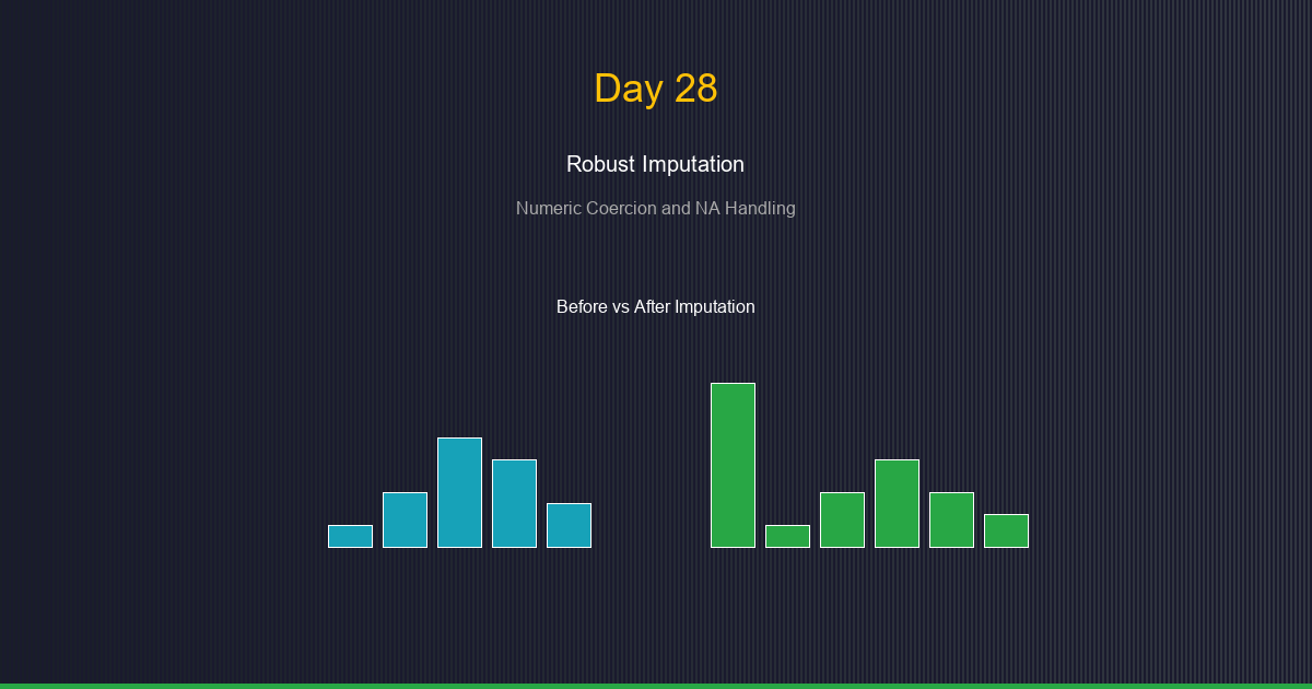
Day 28: Robust Imputation and Numeric Coercion
Understand how data preprocessing choices affect your distributions and downstream thresholds.
Before rules can be evaluated, data must be clean. How you handle missing values and convert data types has profound effects on the distributions your thresholds are based on.
The Problem: Missing Data and Type Mismatches
Scenario: Your fraud detection pipeline receives raw data with:
- Missing values (NA, NULL, "")
- Mixed types ("100", 100, "N/A")
- Invalid entries ("error", -999)
Questions:
- How do you convert everything to numeric?
- What do you replace missing values with?
- How do these choices affect thresholds?
The answer matters more than you think!
Numeric Coercion
What is Coercion?
Coercion is converting data from one type to another.
Common scenarios:
- String → Number: "100" → 100
- Number → Integer: 100.7 → 100 or 101
- Invalid → NA: "error" → NA
Coercion in Practice
Show code (9 lines)
def safe_numeric(value, default=None):
"""
Safely convert to numeric with fallback.
"""
try:
return float(value)
except (ValueError, TypeError):
return default
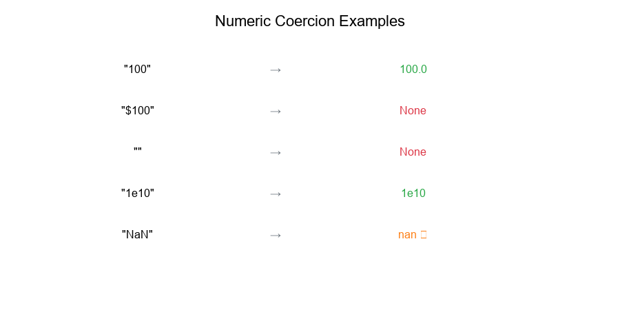
Edge Cases
What happens with:
safe_numeric("100")      # → 100.0
safe_numeric("$100")     # → None (or clean first)
safe_numeric("")         # → None
safe_numeric(None)       # → None
safe_numeric("1e10")     # → 10000000000.0
safe_numeric("NaN")      # → nan (careful!)
Visual Example:
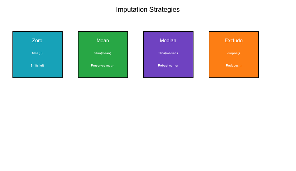
Imputation Strategies
Strategy 1: Impute with Zero
Method: Replace NA with 0
df['amount'] = df['amount'].fillna(0)
When appropriate:
- NA genuinely means "no activity"
- Zero is a valid value in the domain
- You want to flag non-activity
Risks:
- Shifts distribution left
- Inflates zero-count
- Can dramatically change quantiles
Strategy 2: Impute with Mean
Method: Replace NA with the column mean
df['amount'] = df['amount'].fillna(df['amount'].mean())
When appropriate:
- Missing at random (MAR)
- Want to preserve mean
- Large sample sizes
Risks:
- Reduces variance
- Can distort relationships
- Ignores missingness pattern
Strategy 3: Impute with Median
Method: Replace NA with the column median
df['amount'] = df['amount'].fillna(df['amount'].median())
When appropriate:
- Skewed distributions
- Outliers present
- Want robust central tendency
Risks:
- Still reduces variance
- Ignores missingness pattern
- May create spike at median
Strategy 4: Keep as NA (Exclude)
Method: Leave missing and handle separately
df_clean = df.dropna(subset=['amount'])
When appropriate:
- Missingness is informative
- Separate rules for missing
- Small fraction missing
Risks:
- Reduces sample size
- Selection bias if not MCAR
Visual Example:
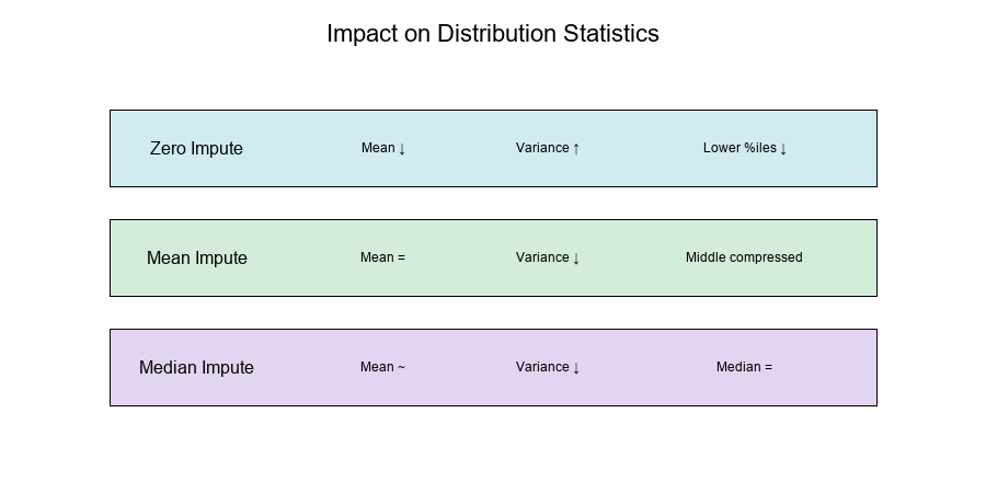
Impact on Distribution Statistics
Mean
Original: μ = Σx_i / n
After zero imputation:
- Mean decreases (zeros pull it down)
- Effect proportional to missing rate
After mean imputation:
- Mean preserved (by design)
- But artificial values added
Variance
Original: σ² = Σ(x_i - μ)² / n
After zero imputation:
- Variance increases if mean > 0
- Creates bimodal distribution
After mean imputation:
- Variance decreases
- Imputed values have zero deviation
Formula for variance reduction:
σ²_new ≈ σ²_old × (1 - missing_rate)
Quantiles
Zero imputation effect:
Original: [10, 20, 30, 40, 50]  → p50 = 30
With 20% zeros: [0, 10, 20, 30, 40, 50]  → p50 = 25 (shifted!)
Median imputation effect:
Original: [10, 20, 30, 40, 50]  → p50 = 30
With imputed 30s: [10, 20, 30, 30, 30, 40, 50]  → p50 = 30 (preserved)
But p75 = 30 (distorted!)
Visual Example:
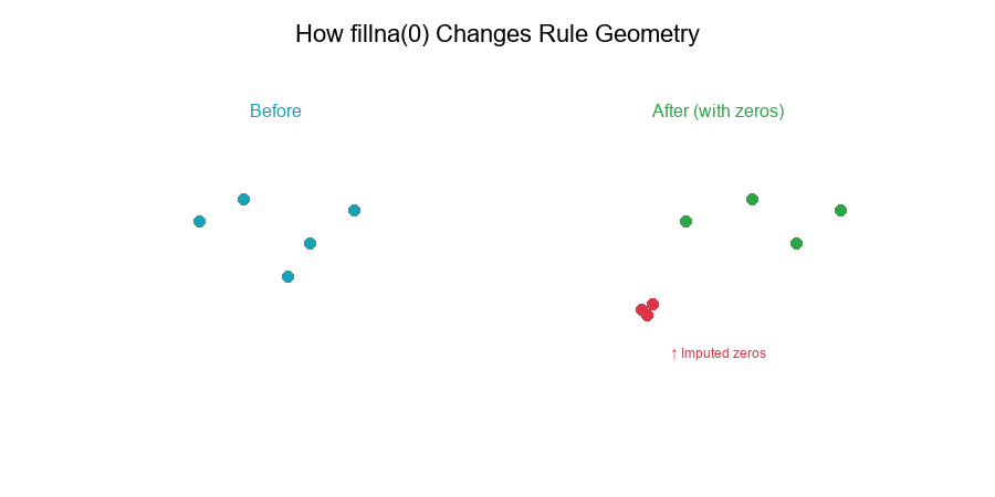
Rule Geometry Changes
How fillna(0) Changes Rules
Before imputation:
Rule: IF amount > threshold THEN flag

Data: [10, 20, NA, 40, 50]
Threshold (p50 excluding NA): 30
Flagged: [40, 50] (2 values)
After fillna(0):
Data: [10, 20, 0, 40, 50]
Threshold (p50): 20  ← Lower!
Flagged: [40, 50] (still 2, but threshold changed)
Geometric Interpretation
In feature space:
- Zero imputation adds points at the origin
- This shifts decision boundaries
- Thresholds based on quantiles move
Example: 2D space
Before: Points scattered in positive quadrant
After: Cluster of zeros at (0, 0)

Decision boundary must now separate:
- True zeros (valid)
- Imputed zeros (missing)
- Positive values
Visual Example:
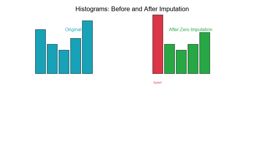
Histograms: Before and After
Visual Comparison
Original distribution (no missing):
0 20 40 60
After zero imputation (20% missing):
0   20   40   60
↑
Spike!
After mean imputation:
0   20   40   60
↑
Spike at mean
Visual Example:
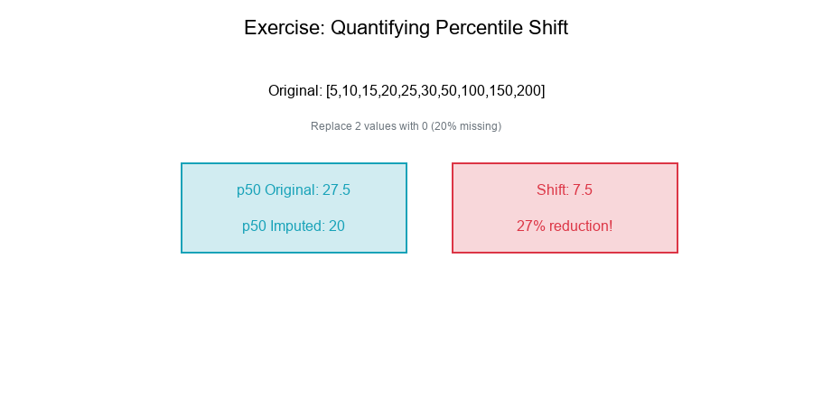
Exercise: Quantifying Percentile Shift
The Problem
Given: A skewed sample with 20% missing values.
Original data (no missing):
[5, 10, 15, 20, 25, 30, 50, 100, 150, 200]
Task: Quantify how replacing 2 random values with NA, then imputing with 0, shifts the 95th percentile.
Solution
Step 1: Original 95th Percentile
data = [5, 10, 15, 20, 25, 30, 50, 100, 150, 200]
p95_original = np.percentile(data, 95)
# p95_original ≈ 187.5 (interpolated)
Step 2: Remove 2 Values (20% missing)
Suppose we remove indices 3 and 7 (values 20 and 100):
data_with_na = [5, 10, 15, NA, 25, 30, 50, NA, 150, 200]
Step 3: Impute with Zero
data_imputed = [5, 10, 15, 0, 25, 30, 50, 0, 150, 200]
Sorted: [0, 0, 5, 10, 15, 25, 30, 50, 150, 200]
Step 4: New 95th Percentile
p95_imputed = np.percentile(data_imputed, 95)
# p95_imputed ≈ 187.5 (high percentile less affected)
Step 5: Effect on Lower Percentiles
p50_original = np.percentile(data, 50)  # ≈ 27.5
p50_imputed = np.percentile(data_imputed, 50)  # ≈ 20

Shift: 27.5 - 20 = 7.5 (27% reduction!)
Key Insights
- High percentiles (90th, 95th): Less affected by zero imputation
- Median (50th): Significantly shifted down
- Lower percentiles (10th, 25th): Pushed to zero
- Effect is proportional to: Missing rate and zero distance from median
Visual Example:
Best Practices for Imputation
1. Understand Your Missing Data
# Analyze missing pattern
missing_rate = df.isna().mean()
missing_correlation = df.isna().corr()
2. Document Your Strategy
IMPUTATION_CONFIG = {
'amount': {'method': 'zero', 'reason': 'NA means no transaction'},
'score': {'method': 'median', 'reason': 'Preserve central tendency'},
'count': {'method': 'exclude', 'reason': 'Analyze separately'},
}
3. Compare Before and After
def imputation_impact_report(original, imputed, percentiles=[25, 50, 75, 90, 95]):
report = {}
for p in percentiles:
orig = np.percentile(original.dropna(), p)
imp = np.percentile(imputed, p)
report[f'p{p}'] = {'original': orig, 'imputed': imp, 'shift': imp - orig}
return report
4. Consider Separate Rules for Missing
if pd.isna(value):
return apply_missing_rule(event)
else:
return apply_normal_rule(event, value)
5. Monitor Drift
Track imputation effects over time as missing patterns change.
6. Use Robust Statistics
When possible, use median-based methods that resist imputation artifacts.
Summary Table
| Strategy | Effect on Mean | Effect on Variance | Effect on Quantiles |
|---|---|---|---|
| Zero | ↓ Decreases | ↑ Increases | ↓ Lower percentiles drop |
| Mean | = Preserved | ↓ Decreases | ~ Middle compressed |
| Median | ~ Slight shift | ↓ Decreases | = Median preserved |
| Exclude | ? Depends | ? Depends | ? Depends on MCAR |
Final Thoughts
Imputation and coercion are not neutral operations—they actively shape your data distribution:
- Zero imputation creates spikes and shifts percentiles down
- Mean/median imputation compresses variance
- Exclusion may introduce selection bias
Key Takeaways:
Coercion must handle edge cases gracefully Zero imputation shifts lower percentiles significantly Mean imputation reduces variance artificially Median imputation is more robust but still affects distribution fillna(0) changes rule geometry by adding origin points Document and monitor your imputation choices
Clean data, clear thresholds!
Where This Shows Up in Practice
- Data Pipelines: Ensuring high-quality filtering and robust statistical metrics before feeding downstream ML models.
- Production Anomaly Detection: Tracking system logs, performance latencies, or transaction volumes under heavy skew.
- A/B Testing & Evaluation: Correctly partitioning user cohorts or comparing treatment outcomes without normal distribution assumptions.