Day 15 — Percentiles as Thresholds: Drawing Lines in the Sand
The Decision-Making Problem
Imagine you're a bank loan officer looking at 10,000 credit applications:
The data:
Credit Scores: 450, 520, 580, 620, 650, 680, 720, 750, 780, 850...
Your job: Draw a line somewhere and decide:
-
Above the line → APPROVE
-
Below the line → REJECT
Questions:
-
Where should that line be?
-
How do we justify the cutoff?
-
What if we want to approve the "top 20%"?
Here's the trick: Percentiles as thresholds!
What Are Percentiles?
Percentile (also called quantile when expressed as proportion):
Definition: The p-th percentile is the value below which p% of the data falls.
Visual Intuition
Imagine 100 people sorted by height:
Show code (10 lines)
Shortest → Tallest

Person 1, 2, 3, ..., 50, ..., 75, ..., 90, ..., 100

10th percentile: Person #10's height (10% are shorter)

50th percentile: Person #50's height (50% are shorter) ← MEDIAN

90th percentile: Person #90's height (90% are shorter)
The core idea: Percentiles divide sorted data into "below" and "above" groups!
Common Percentiles You Know
The Classic Names
Show code (10 lines)
0th percentile   = Minimum

25th percentile  = Q₁ (First Quartile)

50th percentile  = Median (Q₂)

75th percentile  = Q₃ (Third Quartile)

100th percentile = Maximum
Business Examples
Income distribution:
10th percentile: $25,000 (10% earn less)

50th percentile: $55,000 (median income)

90th percentile: $150,000 (top 10% starts here)

99th percentile: $500,000 (the 1%!)
Test scores:
10th percentile: 45 (struggling students)

50th percentile: 72 (average)

90th percentile: 92 (top performers)
Website load times:
50th percentile: 1.2 seconds (typical user)

95th percentile: 3.5 seconds (slow experience)

99th percentile: 8.0 seconds (really bad!)
The Math: Quantile Function
Percentile Definition (Precise)
For data x₁, x₂, ..., xₙ (sorted in ascending order):
The p-th percentile (where p is between 0 and 100):
Show code (10 lines)
Position = (p/100) × (n + 1)

If position is an integer k:

Percentile = xₖ

If position = k + fraction:

Percentile = xₖ + fraction × (xₖ₊₁ - xₖ)  [Linear interpolation]
Example Calculation
Data: [10, 20, 30, 40, 50, 60, 70, 80, 90, 100] (n = 10)
Find 25th percentile (Q₁):
Show code (16 lines)
Position = (25/100) × (10 + 1) = 0.25 × 11 = 2.75

This is between position 2 and 3:

x₂ = 20

x₃ = 30

Q₁ = 20 + 0.75 × (30 - 20)

= 20 + 0.75 × 10

= 20 + 7.5

= 27.5
Find 50th percentile (Median):
Show code (14 lines)
Position = (50/100) × 11 = 5.5

Between position 5 and 6:

x₅ = 50

x₆ = 60

Median = 50 + 0.5 × (60 - 50)

= 50 + 5

= 55
Find 75th percentile (Q₃):
Show code (14 lines)
Position = (75/100) × 11 = 8.25

Between position 8 and 9:

x₈ = 80

x₉ = 90

Q₃ = 80 + 0.25 × (90 - 80)

= 80 + 2.5

= 82.5
Quantile Function Notation
Q(p) = quantile function at proportion p (where p ∈ [0, 1])
Q(0.25) = 25th percentile = Q₁

Q(0.50) = 50th percentile = Median

Q(0.75) = 75th percentile = Q₃
Key property: Q(p) is monotone increasing
If p₁ < p₂, then Q(p₁) ≤ Q(p₂)

Translation: Higher percentiles always give higher (or equal) values! ↗
Using Percentiles as Thresholds
The Decision Framework
Goal: Create decision rules based on data distribution
Method: Pick a percentile → That's your cutoff!
Example: Loan Approval
Data: 10,000 credit scores ranging from 300 to 850
Strategy 1: Approve top 20%
Show code (10 lines)
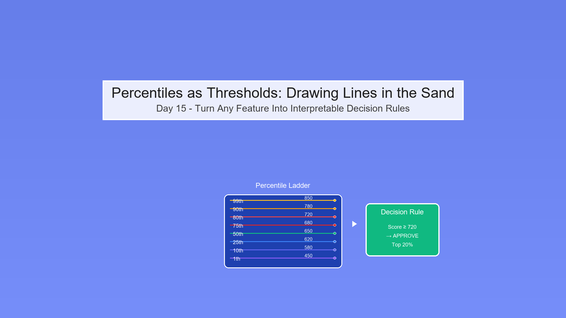
Threshold = 80th percentile

Calculate Q(0.80) = 720

Rule: If credit score ≥ 720 → APPROVE

If credit score < 720 → REJECT

Result: Exactly 20% of applicants approved
Strategy 2: Conservative approach (top 10%)
Show code (10 lines)
Threshold = 90th percentile

Calculate Q(0.90) = 780

Rule: If credit score ≥ 780 → APPROVE

If credit score < 780 → REJECT

Result: Only 10% approved (more selective!)
Strategy 3: Aggressive approach (top 50%)
Show code (10 lines)
Threshold = 50th percentile (median)

Calculate Q(0.50) = 650

Rule: If credit score ≥ 650 → APPROVE

If credit score < 650 → REJECT

Result: Half of applicants approved
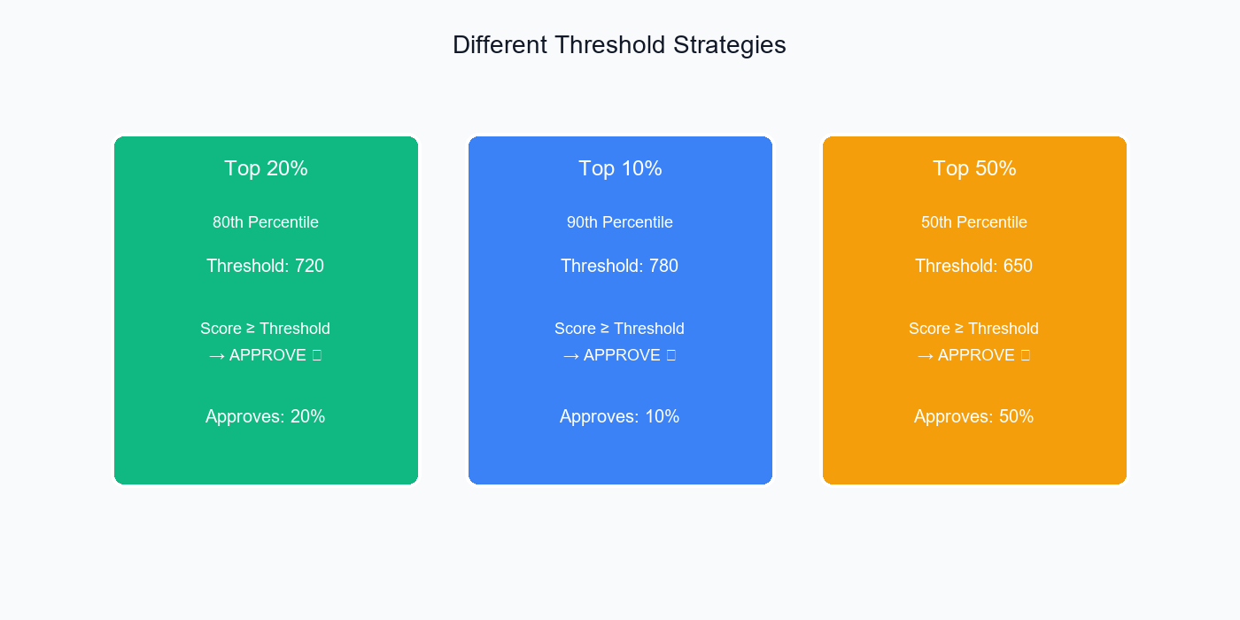
Different threshold strategies yield different approval rates—choose based on your risk tolerance and business goals.
Try It: Interactive Threshold Tuner
Percentile Threshold Tuner
Pick a percentile to set a decision threshold. See how the acceptance rate changes if you approve scores above the threshold.
Visual: Percentile Ladder
Show code (22 lines)
Credit Score Distribution (10,000 applicants)

850  99th percentile (top 1%)

780  90th percentile (top 10%)

720  80th percentile (top 20%)

680  75th percentile (Q₃)

650  50th percentile (Median)

620  25th percentile (Q₁)

580  20th percentile

520  10th percentile

450  1st percentile (bottom 1%)

Pick your rung on the ladder = Pick your threshold!
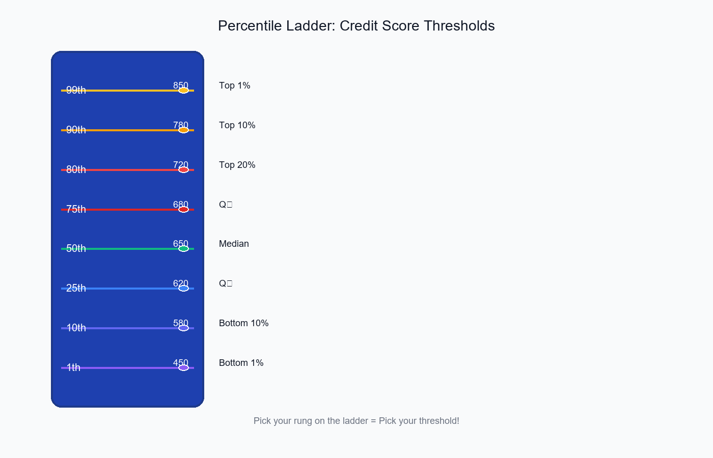
The percentile ladder shows how different thresholds correspond to different approval rates—pick your rung!
Why Percentiles? The Benefits
1. Distribution-Free (Nonparametric)
No assumptions needed!
Show code (10 lines)
Don't need: Normality, specific distribution shape

Works for: Any distribution (skewed, multimodal, weird!)

Example: Income data (highly skewed)

→ Mean = $120K (pulled up by billionaires)

→ 80th percentile = $95K (robust, interpretable)
2. Interpretable
Everyone understands rankings!
"We approve the top 20%"

vs

"We approve scores ≥ 1.5 standard deviations above mean"

Which is clearer? The first!
3. Robust to Outliers
Extreme values don't affect percentiles much:
Show code (12 lines)
Data: [10, 20, 30, 40, 50, 60, 70, 80, 90, 100]

75th percentile = 82.5

Change 100 → 10,000 (outlier!):

Data: [10, 20, 30, 40, 50, 60, 70, 80, 90, 10000]

75th percentile = 82.5 (unchanged!)

The median and nearby percentiles are stable!
4. Direct Control Over Approval Rate
Want to approve 15% of applicants?
Simply set threshold = 85th percentile

Guaranteed to approve exactly 15%!
With parametric methods (z-scores):
z > 1.96 → What % does this approve?

Depends on the distribution!

Need calculations, assumptions, uncertainty...
5. Easy to Adjust
Market changes, need to approve more loans?
Before: 80th percentile (top 20%)

After: 70th percentile (top 30%)

Just slide the threshold down! Simple.
The Monotonicity Property
Theorem: For any dataset, Q(p) is a monotone increasing function.
Formal statement:
If p₁ < p₂, then Q(p₁) ≤ Q(p₂)

In words: Higher percentile → Higher (or equal) threshold value
Why This Matters
Consequence 1: Predictable behavior
If you increase the percentile, the cutoff can ONLY go up (or stay same)

Never goes down!
Consequence 2: Nested approval sets
Show code (10 lines)
People approved at 90th percentile

⊆ People approved at 80th percentile

⊆ People approved at 70th percentile

Top 10% ⊆ Top 20% ⊆ Top 30%

More selective thresholds are subsets!
Consequence 3: Safe threshold adjustment
Increasing percentile → Fewer approvals → Lower risk

Decreasing percentile → More approvals → Higher risk

Direction is guaranteed!
Exercise: Prove Monotonicity
Claim: For sorted data x₁ ≤ x₂ ≤ ... ≤ xₙ, if p₁ < p₂, then Q(p₁) ≤ Q(p₂)
Proof:
Case 1: Integer Positions
Setup:
Show code (10 lines)
Position for p₁: k₁ = ⌊(p₁/100) × (n+1)⌋

Position for p₂: k₂ = ⌊(p₂/100) × (n+1)⌋

Since p₁ < p₂:

(p₁/100) × (n+1) < (p₂/100) × (n+1)

Therefore: k₁ ≤ k₂
Since data is sorted (x₁ ≤ x₂ ≤ ... ≤ xₙ):
Show code (10 lines)
Q(p₁) = xₖ₁

Q(p₂) = xₖ₂

Since k₁ ≤ k₂ and data is sorted:

xₖ₁ ≤ xₖ₂

Therefore: Q(p₁) ≤ Q(p₂)
Case 2: Non-Integer Positions (Interpolation)
Setup:
Position for p₁: pos₁ = (p₁/100) × (n+1) = k₁ + f₁

Position for p₂: pos₂ = (p₂/100) × (n+1) = k₂ + f₂

Where k₁, k₂ are integer parts, f₁, f₂ are fractional parts
Interpolation formula:
Q(p₁) = xₖ₁ + f₁ × (xₖ₁₊₁ - xₖ₁)

Q(p₂) = xₖ₂ + f₂ × (xₖ₂₊₁ - xₖ₂)
Sub-case 2a: k₁ = k₂ (same interval)
Show code (14 lines)
If k₁ = k₂ and p₁ < p₂:

Then pos₁ < pos₂, so f₁ < f₂

Q(p₁) = xₖ + f₁ × (xₖ₊₁ - xₖ)

Q(p₂) = xₖ + f₂ × (xₖ₊₁ - xₖ)

Since f₁ < f₂ and (xₖ₊₁ - xₖ) ≥ 0 (sorted):

f₁ × (xₖ₊₁ - xₖ) ≤ f₂ × (xₖ₊₁ - xₖ)

Therefore: Q(p₁) ≤ Q(p₂)
Sub-case 2b: k₁ < k₂ (different intervals)
Show code (10 lines)
Since k₁ < k₂ and data sorted:

xₖ₁ ≤ xₖ₂

Also, since 0 ≤ f₁, f₂ < 1:

xₖ₁ ≤ xₖ₁ + f₁ × (xₖ₁₊₁ - xₖ₁) ≤ xₖ₁₊₁ ≤ ... ≤ xₖ₂

Therefore: Q(p₁) ≤ Q(p₂)
Conclusion: In all cases, Q(p₁) ≤ Q(p₂) when p₁ < p₂!
Practical Demonstration
Data: [10, 15, 20, 25, 30, 35, 40, 45, 50, 55] (n=10)
Test increasing percentiles:
Show code (9 lines)
import numpy as np

data = [10, 15, 20, 25, 30, 35, 40, 45, 50, 55]
percentiles = [10, 20, 30, 40, 50, 60, 70, 80, 90]

for p in percentiles:
threshold = np.percentile(data, p)
print(f"{p}th percentile: {threshold}")
Output:
Show code (20 lines)
10th percentile: 10.5

20th percentile: 13.0    (≥ 10.5)

30th percentile: 17.0    (≥ 13.0)

40th percentile: 23.0    (≥ 17.0)

50th percentile: 30.0    (≥ 23.0)

60th percentile: 37.0    (≥ 30.0)

70th percentile: 42.0    (≥ 37.0)

80th percentile: 47.0    (≥ 42.0)

90th percentile: 52.0    (≥ 47.0)

Every step up in percentile → threshold increases (or stays same)!
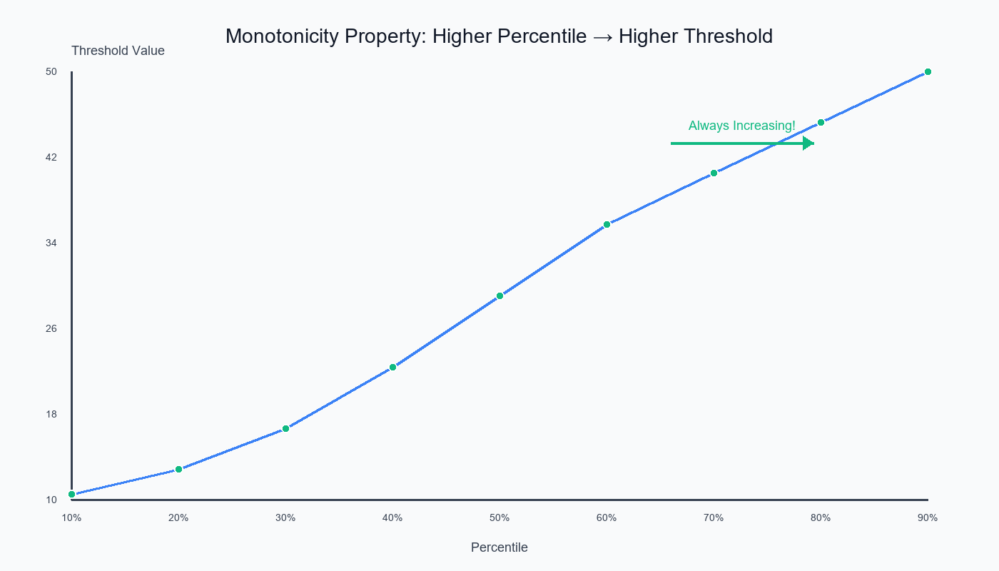
The monotonicity property ensures that higher percentiles always yield higher (or equal) threshold values—guaranteed!
Implementation: compute_percentile_thresholds
Show code (53 lines)
import numpy as np
import pandas as pd

def compute_percentile_thresholds(data, percentiles=[25, 50, 75, 90, 95, 99]):
"""
Compute threshold values at specified percentiles

Parameters:
- data: array-like, feature values
- percentiles: list of percentiles to compute

Returns:
- DataFrame with percentiles and corresponding thresholds
"""

# Sort data for visualization
sorted_data = np.sort(data)
n = len(data)

results = []

for p in percentiles:
# Compute threshold
threshold = np.percentile(data, p)

# Count values above and below
n_below = np.sum(data < threshold)
n_above = np.sum(data >= threshold)

# Percentage above (approval rate if used as cutoff)
pct_above = (n_above / n) * 100

results.append({
'percentile': p,
'threshold': threshold,
'n_below': n_below,
'n_above': n_above,
'approval_rate_%': pct_above
})

return pd.DataFrame(results)

# Example usage
np.random.seed(42)
credit_scores = np.random.normal(650, 100, 10000).clip(300, 850)

thresholds_df = compute_percentile_thresholds(
credit_scores,
percentiles=[50, 75, 80, 85, 90, 95, 99]
)

print(thresholds_df)
Output:
Show code (16 lines)
percentile  threshold  n_below  n_above  approval_rate_%

0          50     649.73     5000     5000            50.00

1          75     717.04     7500     2500            25.00

2          80     733.56     8000     2000            20.00

3          85     751.39     8500     1500            15.00

4          90     777.82     9000     1000            10.00

5          95     814.56     9500      500             5.00

6          99     882.19     9900      100             1.00
Interpretation:
-
Want to approve 20%? Set threshold at 733.56 (80th percentile)
-
Want top 5%? Set threshold at 814.56 (95th percentile)
Visualizing Percentile Thresholds
Percentile Ladder on Histogram
Show code (40 lines)
import matplotlib.pyplot as plt

def visualize_percentile_thresholds(data, percentiles=[50, 75, 90, 95]):
"""
Visualize data distribution with percentile thresholds marked
"""
fig, ax = plt.subplots(figsize=(12, 6))

# Histogram
ax.hist(data, bins=50, alpha=0.6, color='skyblue', edgecolor='black')

# Add percentile lines
colors = ['green', 'orange', 'red', 'darkred']

for p, color in zip(percentiles, colors):
threshold = np.percentile(data, p)
ax.axvline(threshold, color=color, linestyle='--', linewidth=2,
label=f'{p}th percentile: {threshold:.1f}')

# Add approval rate annotation
approval_rate = 100 - p
ax.text(threshold, ax.get_ylim()[1]*0.9,
f'Top {approval_rate:.0f}%',
rotation=90, verticalalignment='bottom',
color=color, fontweight='bold')

ax.set_xlabel('Credit Score', fontsize=12)
ax.set_ylabel('Frequency', fontsize=12)
ax.set_title('Credit Score Distribution with Percentile Thresholds',
fontsize=14, fontweight='bold')
ax.legend(loc='upper left')
ax.grid(alpha=0.3)

plt.tight_layout()
return fig

# Generate and plot
fig = visualize_percentile_thresholds(credit_scores, [50, 75, 85, 90, 95])
plt.show()
Sorted Values with Percentile Markers
Show code (38 lines)
def plot_sorted_with_percentiles(data, percentiles=[25, 50, 75, 90, 95]):
"""
Plot sorted data values with percentile positions marked
"""
sorted_data = np.sort(data)
n = len(data)

fig, ax = plt.subplots(figsize=(12, 6))

# Plot sorted values
ax.plot(range(n), sorted_data, color='blue', alpha=0.5, linewidth=1)

# Mark percentiles
colors = ['green', 'yellow', 'orange', 'red', 'darkred']

for p, color in zip(percentiles, colors):
threshold = np.percentile(data, p)
position = int((p/100) * n)

ax.scatter(position, threshold, color=color, s=200,
zorder=5, edgecolor='black', linewidth=2)
ax.axhline(threshold, color=color, linestyle=':', alpha=0.5)
ax.text(n*0.02, threshold, f'{p}th: {threshold:.1f}',
fontsize=10, color=color, fontweight='bold',
bbox=dict(boxstyle='round', facecolor='white', alpha=0.8))

ax.set_xlabel('Rank (sorted position)', fontsize=12)
ax.set_ylabel('Credit Score', fontsize=12)
ax.set_title('Sorted Credit Scores with Percentile Markers',
fontsize=14, fontweight='bold')
ax.grid(alpha=0.3)

plt.tight_layout()
return fig

fig = plot_sorted_with_percentiles(credit_scores)
plt.show()
Visual shows:
Show code (22 lines)
Credit Score

850                                           • 99th

800                                     • 95th

750                              • 90th

700                       • 75th

650              • 50th

600        • 25th

•

300 → Rank

0         2500      5000      7500    10000

The curve shows monotonicity visually!
Advanced: Percentile-at-Value
Sometimes you want the reverse: "What percentile is this score?"
Show code (26 lines)
def compute_percentile_at_value(data, value):
"""
Compute what percentile a given value corresponds to

Parameters:
- data: array-like
- value: scalar value to find percentile for

Returns:
- percentile: where this value falls (0-100)
"""
n = len(data)
n_below = np.sum(data < value)
n_equal = np.sum(data == value)

# Midpoint method: count half of ties
percentile = ((n_below + n_equal/2) / n) * 100

return percentile

# Example
score = 720
percentile = compute_percentile_at_value(credit_scores, score)
print(f"A score of {score} is at the {percentile:.1f}th percentile")
print(f"This is better than {percentile:.1f}% of applicants")
Output:
A score of 720 is at the 75.3th percentile

This is better than 75.3% of applicants
Use cases:
-
"You scored 720, which beats 75% of applicants!"
-
"This transaction is at the 99.5th percentile for amount"
-
"Your response time is at the 5th percentile (very fast!)"
When to Use Percentile Thresholds
Perfect For:
Quota-based decisions
"Approve top 1,000 applicants"

→ Use 90th percentile (10% of 10,000)
Relative performance
"Bonus for top 20% performers"

→ Use 80th percentile of sales
Anomaly detection
"Flag transactions above 99th percentile"

→ Catches unusual amounts
Resource allocation
"Prioritize cases in top 30% of urgency"

→ Use 70th percentile of urgency score
SLA definitions
"95% of requests must complete under X seconds"

→ Use 95th percentile as threshold
Don't Use When:
Absolute standards matter
"Approve everyone with score > 700"

Not: "Approve top 20%"

If the standard is fixed, percentiles aren't appropriate!
Small sample sizes
n = 10: Percentiles unstable

Better: Use all data or simple cutoffs
Need theoretical justification
"Why 80th percentile?"

"Because... we decided?"

Percentiles are data-driven but somewhat arbitrary
Distribution is important
If you specifically need Normal(μ, σ) behavior

Percentiles don't preserve distributional properties
Combining Percentiles with Business Logic
Example: Risk-Adjusted Approval
Show code (31 lines)
def tiered_approval_thresholds(credit_score, income,
credit_percentiles, income_percentiles):
"""
Use percentiles from both features for tiered decisions

Tiers:
- Tier 1 (Auto-approve): Both top 25%
- Tier 2 (Manual review): One top 25%
- Tier 3 (Auto-reject): Neither top 25%
"""

credit_pct = compute_percentile_at_value(credit_scores_data, credit_score)
income_pct = compute_percentile_at_value(income_data, income)

if credit_pct >= 75 and income_pct >= 75:
return "APPROVED", "Tier 1: Excellent on both metrics"
elif credit_pct >= 75 or income_pct >= 75:
return "REVIEW", "Tier 2: Strong on one metric"
else:
return "REJECTED", "Tier 3: Below threshold on both"

# Example
decision, reason = tiered_approval_thresholds(
credit_score=750,  # 85th percentile
income=80000,      # 60th percentile
credit_percentiles=credit_scores,
income_percentiles=incomes
)
print(f"Decision: {decision}")
print(f"Reason: {reason}")
Output:
Decision: REVIEW

Reason: Tier 2: Strong on one metric
Common Pitfalls
1. Ties at Percentile
Show code (12 lines)
Data: [10, 20, 20, 20, 30, 40, 50, 60, 70, 80]

↑_____↑

Three 20's

50th percentile falls in the middle of ties!

Different software may handle differently.

Solution: Be consistent, document method
2. Small Sample Instability
Show code (14 lines)
n = 10:

99th percentile = ???

Position = 0.99 × 11 = 10.89

Interpolation between 10th and... 11th value?

There is no 11th value!

Solution: Use percentiles < 100 × (n-1)/n

For n=10: Max reliable percentile ≈ 90%
3. Assuming Equal Intervals
Show code (20 lines)
Wrong thinking:

"50th and 75th are 25 points apart

So 50th to 25th are also 25 points apart"

Reality:

Percentiles mark equal COUNTS, not equal VALUES

Data: [1, 2, 3, 100]

25th percentile: 1.75

50th percentile: 2.50

75th percentile: 51.25

Look at those gaps! Not equal!
4. Confusing Percentile and Percentage
"Score at 80th percentile = 80% correct"

"Score at 80th percentile = Better than 80% of people"

Very different!
5. Using Percentiles on Small Subgroups
Show code (16 lines)
Total data: n = 10,000

Subgroup: n = 50

Computing 99th percentile on subgroup:

Position = 0.99 × 51 = 50.49

You're asking for the 50th value in a group of 50!

Basically the maximum. Unreliable!

Solution: Use percentiles from full data,

apply to subgroups
Summary
Percentiles are powerful, interpretable threshold proposals that require no distributional assumptions!
Key Concepts:
Percentile definition: Value below which p% of data falls
p-th percentile = Q(p/100)
Quantile function Q(p): Inverse of CDF, maps [0,1] → data values
Monotonicity property:
If p₁ < p₂, then Q(p₁) ≤ Q(p₂)

Higher percentile → Higher (or equal) threshold ↗
As decision threshold:
Want top 20%? Use 80th percentile

Guaranteed to select exactly 20%!
Robust & nonparametric:
-
No normal assumption needed
-
Stable to outliers
-
Works with any distribution
The Monotonicity Proof:
For sorted data x₁ ≤ x₂ ≤ ... ≤ xₙ:
Show code (10 lines)
p₁ < p₂

→ Position(p₁) < Position(p₂)

→ xₖ₁ ≤ xₖ₂  (because sorted)

→ Q(p₁) ≤ Q(p₂)

Increasing percentile ALWAYS increases threshold!
When to Use:
Quota-based decisions ("top 10%")
Relative rankings ("better than 75%")
Anomaly detection ("above 99th percentile")
SLA definitions ("95% under threshold")
Data-driven threshold proposals
Fixed absolute standards ("must score > 700")
Small samples (n < 50)
Theoretical distribution requirements
Implementation:
Show code (9 lines)
# Compute thresholds
thresholds = compute_percentile_thresholds(data, [75, 90, 95])

# Find percentile of value
pct = compute_percentile_at_value(data, 720)

# Use as decision rule
approved = data >= np.percentile(data, 80)  # Top 20%
The power: Turn any feature into an interpretable, ranked decision threshold without complex modeling!
Note: This article uses technical terms like percentiles, quantiles, thresholds, monotonicity, and nonparametric. For definitions, check out the Key Terms & Glossary page.