Day 29: Putting It All Together - Constructing a Stratified Audit Plan
Synthesize quantile thresholds, stratification, sample sizes, and investigation workflows into a complete audit plan.
We've built the mathematical foundations. Now it's time to assemble them into a complete stratified audit plan—from threshold computation to sample selection to investigation summary.
The Goal: End-to-End Audit Plan
Objective: Design a stratified sampling plan that:
- Partitions population into meaningful strata
- Allocates samples optimally across strata
- Enables statistical inference about fraud rates
- Provides actionable investigation priorities
Key Components:
Threshold Computation → Stratification → Sample Sizing →
Selection → Investigation → Summary → Adjustment
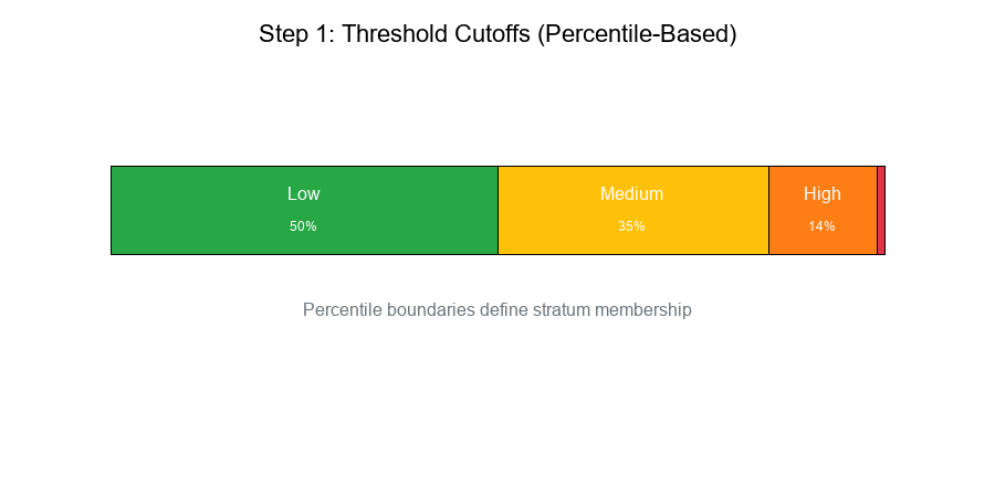
Step 1: Threshold Computation
Using Quantile-Based Cutoffs
Approach: Use percentiles to define stratum boundaries.
Example: Transaction Amount Strata
Show code (9 lines)
# Compute percentile cutoffs
data = transactions['amount']
cutoffs = {
'Low': (0, np.percentile(data, 50)),           # 0-50th percentile
'Medium': (np.percentile(data, 50), np.percentile(data, 85)),  # 50-85th
'High': (np.percentile(data, 85), np.percentile(data, 99)),    # 85-99th
'Extreme': (np.percentile(data, 99), np.inf)   # 99th+
}
Result:
Show code (9 lines)
Stratum     Range           Count    % of Population

Low         $0 - $100       50,000   50%
Medium      $100 - $500     35,000   35%
High        $500 - $2,000   14,000   14%
Extreme     $2,000+          1,000    1%

Total                      100,000  100%
Visual Example:
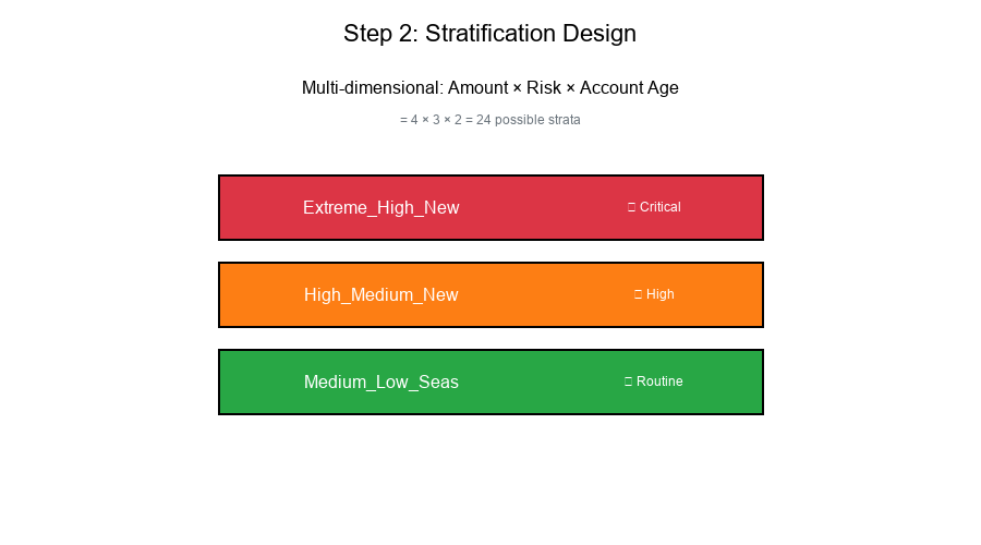
Step 2: Stratification Design
Combining Multiple Features
Multi-dimensional stratification:
Show code (14 lines)
def create_strata(df):
"""
Create strata based on multiple features.
"""
strata = []

for amount_level in ['Low', 'Medium', 'High', 'Extreme']:
for risk_level in ['Low', 'Medium', 'High']:
for account_age in ['New', 'Seasoned']:
stratum = f"{amount_level}_{risk_level}_{account_age}"
strata.append(stratum)

return strata  # 4 × 3 × 2 = 24 strata
Stratum Characteristics
For each stratum, compute:
- Population size (N_h): Number of elements
- Expected fraud rate (p_h): Historical or estimated
- Variance (σ²_h): Variability within stratum
- Cost per sample (c_h): Investigation cost
Example Table:
Show code (9 lines)
Stratum              N_h     p_h     σ²_h    Priority

Extreme_High_New     200     0.15    0.13     Critical
Extreme_High_Seas    150     0.08    0.07     High
High_High_New        500     0.12    0.11     Critical
High_Medium_New      800     0.06    0.06     High
Medium_Low_Seas    10000     0.01    0.01     Routine
Low_Low_Seas       35000     0.002   0.002    Routine
Visual Example:
Step 3: Sample Size Determination
Power Analysis Framework
Goal: Determine sample size n_h for each stratum to detect fraud rate p_h with desired power.
Using Day 14 concepts:
Show code (21 lines)
def required_sample_size(p_h, p_0, alpha=0.05, power=0.80):
"""
Sample size for detecting deviation from baseline.

p_h: Expected fraud rate in stratum
p_0: Null hypothesis rate
alpha: Significance level
power: Desired power (1 - β)
"""
from scipy import stats

z_alpha = stats.norm.ppf(1 - alpha/2)
z_beta = stats.norm.ppf(power)

effect = p_h - p_0
pooled_var = p_h * (1 - p_h) + p_0 * (1 - p_0)

n = ((z_alpha + z_beta)**2 * pooled_var) / (effect**2)

return int(np.ceil(n))
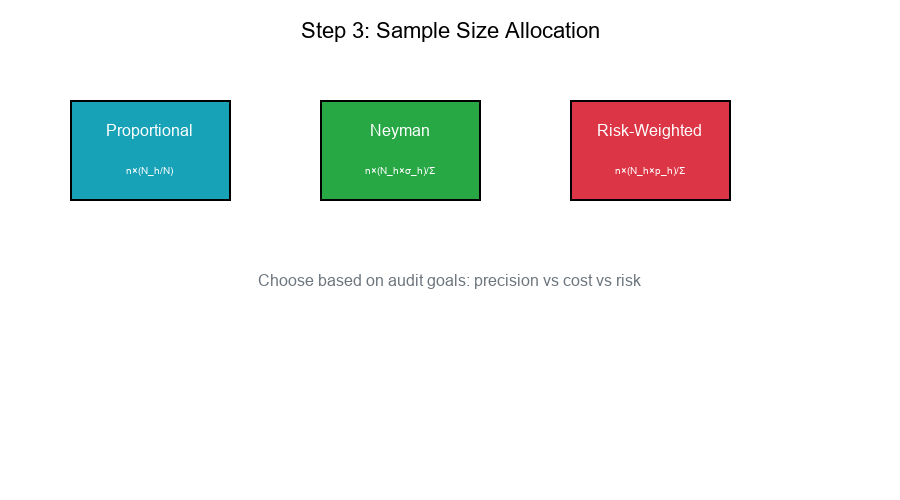
Allocation Strategies
Proportional Allocation:
n_h = n × (N_h / N)
Neyman Allocation (optimal for variance):
n_h = n × (N_h × σ_h) / Σ(N_j × σ_j)
Risk-Weighted Allocation:
n_h = n × (N_h × p_h) / Σ(N_j × p_j)
Sample Size Table
Show code (11 lines)
Stratum              N_h     p_h     Proportional  Neyman    Risk-Weighted

Extreme_High_New     200     0.15         2          15          50
Extreme_High_Seas    150     0.08         2          10          20
High_High_New        500     0.12         5          35          100
High_Medium_New      800     0.06         8          30          80
Medium_Low_Seas    10000     0.01        100         50          167
Low_Low_Seas       35000     0.002       350         20          117

Total Sample         n       -          467         160         534
Visual Example:
Step 4: Sample Selection
Random Selection Within Strata
Show code (20 lines)
def select_stratified_sample(df, strata_col, sample_sizes):
"""
Select random samples from each stratum.
"""
samples = []

for stratum, n in sample_sizes.items():
stratum_data = df[df[strata_col] == stratum]

if len(stratum_data) <= n:
# Take all if stratum is small
sample = stratum_data
else:
# Random sample
sample = stratum_data.sample(n=n, random_state=42)

samples.append(sample)

return pd.concat(samples)
Selection Tracking
selection_log = {
'stratum': [],
'population_size': [],
'sample_size': [],
'sampling_fraction': [],
'selection_date': [],
}
Step 5: Investigation Workflow
Investigation Priority Queue
Show code (22 lines)
def prioritize_investigations(sample, priority_rules):
"""
Assign investigation priority based on rules.
"""
priorities = []

for idx, row in sample.iterrows():
# Apply priority rules
if row['stratum'].startswith('Extreme_High'):
priority = 1  # Immediate
elif row['stratum'].startswith('High_High'):
priority = 2  # Urgent
elif 'High' in row['stratum']:
priority = 3  # Standard
else:
priority = 4  # Routine

priorities.append(priority)

sample['priority'] = priorities
return sample.sort_values('priority')
Investigation Outcomes
Track for each case:
- Confirmed Fraud (True Positive)
- Legitimate (False Positive)
- Inconclusive
- Time to resolution
Step 6: Summary and Reporting
Stratum-Level Summary
Show code (15 lines)
def investigation_summary(results):
"""
Summarize investigation results by stratum.
"""
summary = results.groupby('stratum').agg({
'is_fraud': ['sum', 'count', 'mean'],
'amount': 'sum',
'resolution_hours': 'mean'
})

summary.columns = ['fraud_count', 'total_reviewed',
'fraud_rate', 'total_amount', 'avg_hours']

return summary
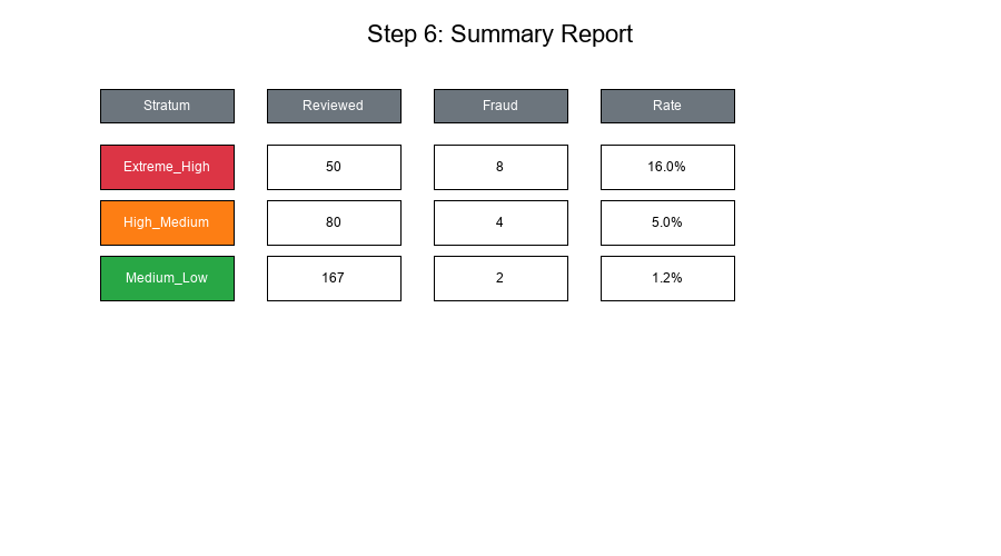
Example Summary Report
Show code (11 lines)
Stratum              Reviewed  Fraud  Rate    Amount      Avg Hours

Extreme_High_New        50       8    16.0%   $125,000      2.5
Extreme_High_Seas       20       2    10.0%    $45,000      2.0
High_High_New          100      10    10.0%   $280,000      3.0
High_Medium_New         80       4     5.0%   $150,000      2.5
Medium_Low_Seas        167       2     1.2%   $200,000      1.5
Low_Low_Seas           117       0     0.0%    $80,000      1.0

TOTAL                  534      26     4.9%   $880,000      2.1
Visual Example:
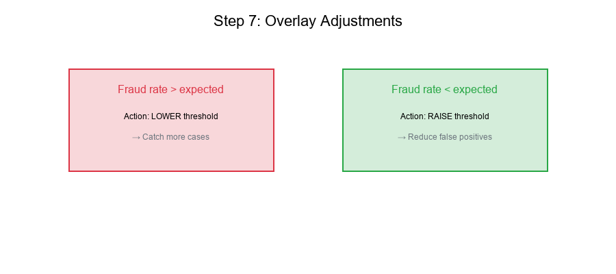
Step 7: Overlay Adjustments
Using Results to Refine Thresholds
Based on investigation findings:
- Adjust cutoffs if fraud rates differ from expected
- Reallocate samples to high-yield strata
- Update priority rules based on actual outcomes
- Refine feature selection for stratification
Adjustment Framework
Show code (25 lines)
def suggest_adjustments(summary, expectations):
"""
Suggest threshold adjustments based on results.
"""
adjustments = []

for stratum, row in summary.iterrows():
expected = expectations.get(stratum, {}).get('fraud_rate', 0.05)
actual = row['fraud_rate']

if actual > expected * 1.5:
adjustments.append({
'stratum': stratum,
'action': 'LOWER_THRESHOLD',
'reason': f'Fraud rate {actual:.1%} >> expected {expected:.1%}'
})
elif actual < expected * 0.5:
adjustments.append({
'stratum': stratum,
'action': 'RAISE_THRESHOLD',
'reason': f'Fraud rate {actual:.1%} << expected {expected:.1%}'
})

return adjustments
Visual Example:
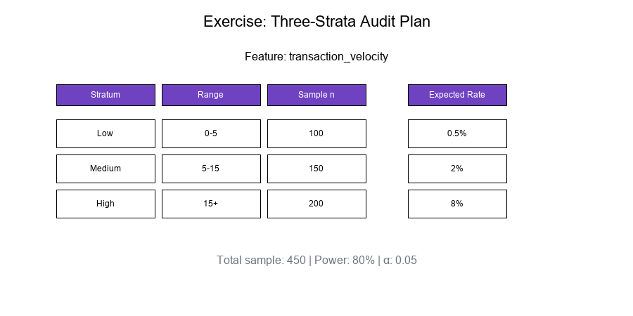
Exercise: Design a Three-Strata Plan
The Problem
Given: A mock feature "transaction_velocity" (transactions per hour)
Design: A three-strata audit plan with:
- Cutoffs (percentile-based)
- Sample sizes (power-based)
- Expected outcomes
Solution
Step 1: Analyze Feature Distribution
velocity_data = [0.5, 1, 2, 3, 5, 8, 10, 15, 20, 50, ...] # n = 10,000
Compute percentiles:
p50 = 5 transactions/hour
p85 = 15 transactions/hour
p99 = 50 transactions/hour
Step 2: Define Strata
| Stratum | Range | N_h | Expected p_h | |---------|-------|-----|--------------| | Low | 0 - 5 | 5,000 | 0.5% | | Medium | 5 - 15 | 3,500 | 2% | | High | 15+ | 1,500 | 8% |
Step 3: Compute Sample Sizes
Using power = 80%, α = 0.05, detecting p_h vs p_0 = 0.5%:
Low:    n = 100 (confirm low rate)
Medium: n = 150 (detect elevation)
High:   n = 200 (estimate accurately)
Total:  n = 450
Step 4: Expected Outcomes
Stratum    Sample    Expected Fraud    Expected Rate

Low        100       0-1               ~0.5%
Medium     150       2-4               ~2%
High       200       14-18             ~8%

Total      450       16-23             ~4%
Step 5: Document the Plan
Show code (14 lines)
audit_plan = {
'feature': 'transaction_velocity',
'strata': [
{'name': 'Low', 'range': (0, 5), 'n': 100, 'priority': 3},
{'name': 'Medium', 'range': (5, 15), 'n': 150, 'priority': 2},
{'name': 'High', 'range': (15, np.inf), 'n': 200, 'priority': 1}
],
'total_sample': 450,
'power': 0.80,
'alpha': 0.05,
'version': '1.0',
'created': '2025-11-29'
}
Visual Example:
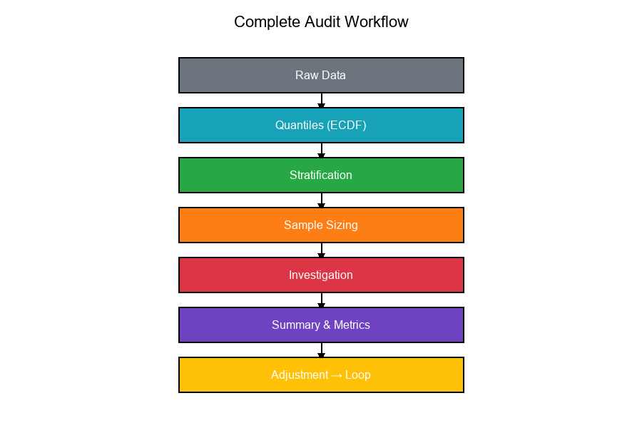
Complete Workflow Flowchart
Show code (20 lines)
Raw Data

Compute Quantiles   Day 13-15: Percentiles, ECDF

Define Strata       Day 23-24: Partitioning, Risk Levels

Compute Sample      Day 14: Power Analysis
Sizes

Select Samples      Day 16: Hypergeometric Sampling

Investigate

Summarize Results   Day 18: F1 Score, Metrics

Adjust Thresholds   Day 22: Set Overlap Analysis

Loop back to refine
Visual Example:
Summary Table
| Step | Input | Output | Key Concepts |
|---|---|---|---|
| 1. Thresholds | Raw data | Percentile cutoffs | Quantiles, ECDF |
| 2. Stratification | Cutoffs | Strata definitions | Partitioning |
| 3. Sample Sizing | Strata, power | n per stratum | Power analysis |
| 4. Selection | Population | Sample | Random sampling |
| 5. Investigation | Sample | Outcomes | Priority queue |
| 6. Summary | Outcomes | Report | Rates, metrics |
| 7. Adjustment | Report | New thresholds | Feedback loop |
Final Thoughts
A stratified audit plan is the culmination of all our mathematical tools:
- Quantiles define stratum boundaries
- Power analysis determines sample sizes
- Stratification enables targeted investigation
- Metrics measure effectiveness
- Feedback loops enable continuous improvement
Key Takeaways:
Quantile thresholds create meaningful strata Sample allocation balances precision and cost Power analysis ensures detectable differences Investigation priority focuses resources Summary reporting enables decisions Overlay adjustments close the loop
Plan stratified, investigate smart!