Day 3 — Percentiles and Quantiles: Understanding Data Distributions 📊

💡 Note: This article uses technical terms and abbreviations. For definitions, check out the Key Terms & Glossary page.

🎯 Introduction

Percentiles and quantiles are fundamental tools for understanding data distributions. They tell us where values sit relative to the rest of the data, providing robust measures that resist outliers and work well with transformations.

TL;DR:

Percentiles describe "how far up the data" a value sits. They come from the empirical CDF (ECDF) and order statistics. They are robust to outliers compared to means, and they behave nicely under monotone transforms (e.g., rescaling). Knowing your quantile definition (interpolation rule) matters because different tools use slightly different formulas.

📘 What is a Percentile?

• The p‑th percentile (e.g., p = 0.8 for the 80th) is a value such that p (≈ 80%) of the data are at or below it.
• We get percentiles from the empirical CDF:
  • ECDF:
    Fₙ(x) = (1/n) · number of sample values ≤ x
  • Quantile (left inverse of CDF):
    Q(p) = inf { x : F(x) ≥ p }
    (for the ECDF, we get an empirical quantile)

In simple terms: sort your data; the p‑th percentile is somewhere at the p‑fraction along that sorted list.

📦 Order Statistics (the building blocks)

• Sort your n values: x(1) ≤ x(2) ≤ … ≤ x(n)
• These sorted values are "order statistics."
• Quantiles are determined by positions along this sorted list (possibly between two entries with interpolation).

✨ Why percentiles are useful

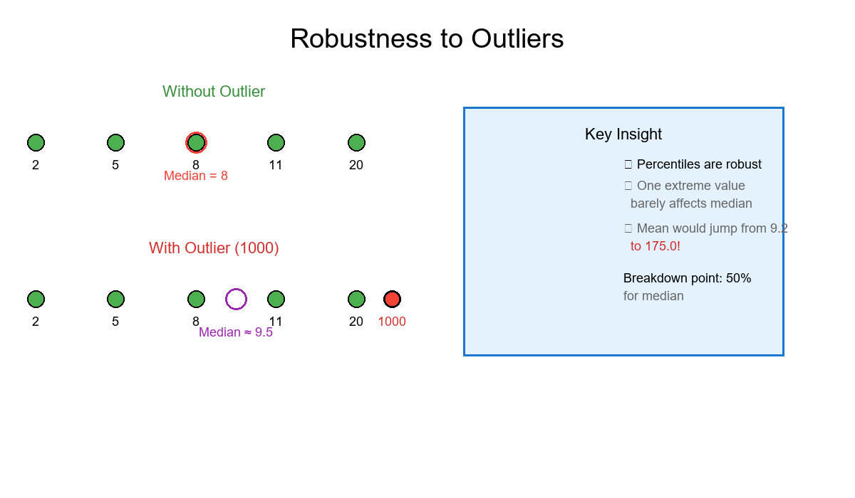
• 🛡️ Robust to outliers: a single extreme value does not change the median or most percentiles.
  (The median has a 50% breakdown point; a general p‑quantile has breakdown min(p, 1−p).)
• 🔄 Invariant to monotone transforms:
  If f is strictly increasing, the quantile of f(X) at p is f(quantile of X at p).
  For example, scaling by a>0 and shifting by b just scales and shifts the quantiles:
  Q_{aX+b}(p) = a · Q_X(p) + b
• 📏 Unit‑free ranks: percentiles depend on ordering, not the units.

🔢 How different tools compute empirical percentiles (interpolation choices)

There isn't just one "empirical percentile." Common choices:

• 1️⃣ Nearest rank (simple): position k = ceil(p·n); quantile = x(k)
• 2️⃣ Linear interpolation between neighbors (popular; e.g., "Type 7"):
  h = 1 + (n−1)·p
  Let j = floor(h), γ = h − j
  Q(p) = (1−γ)·x(j) + γ·x(j+1)

Other "types" shift where they anchor ranks, but the key point is: pick and stick to one method for consistency.

🧩 Solved example 1 — 20th and 80th percentiles (nearest rank and Type 7)

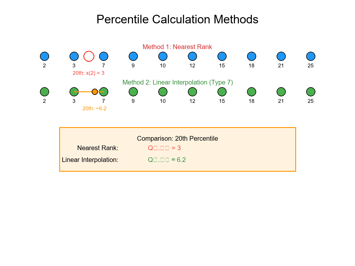
Data (unsorted):
[12, 3, 7, 9, 25, 18, 2, 15, 21, 10]
Sorted:
x = [2, 3, 7, 9, 10, 12, 15, 18, 21, 25] (n = 10)

A) Nearest rank

• 20th percentile (p = 0.20): k = ceil(0.20·10) = ceil(2) = 2 → x(2) = 3
• 80th percentile (p = 0.80): k = ceil(0.80·10) = ceil(8) = 8 → x(8) = 18

Nearest-rank answers:
Q₀.₂₀ = 3, Q₀.₈₀ = 18

B) Linear interpolation (Type 7, used by many libraries)

• 20th percentile:
  h = 1 + (n−1)·p = 1 + 9·0.20 = 2.8
  j = floor(2.8) = 2, γ = 0.8
  Q₀.₂₀ = (1−0.8)·x(2) + 0.8·x(3) = 0.2·3 + 0.8·7 = 0.6 + 5.6 = 6.2
• 80th percentile:
  h = 1 + 9·0.80 = 8.2
  j = 8, γ = 0.2
  Q₀.₈₀ = 0.8·x(8) + 0.2·x(9) = 0.8·18 + 0.2·21 = 14.4 + 4.2 = 18.6

Type‑7 answers:
Q₀.₂₀ ≈ 6.2, Q₀.₈₀ ≈ 18.6

Note how the method changes the number. That's normal; document your method.

🔗 Solved example 2 — Duplicates and ties

Data: [5, 5, 5, 7, 9] (n = 5)
Sorted: [5, 5, 5, 7, 9]

• Nearest rank 20th (p=0.2): k=ceil(0.2·5)=ceil(1)=1 → 5

• Nearest rank 80th (p=0.8): k=ceil(0.8·5)=ceil(4)=4 → 7

• Type 7 20th: h=1+(4·0.2)=1.8 → j=1, γ=0.8 → Q=0.2·x(1)+0.8·x(2)=0.2·5+0.8·5=5

• Type 7 80th: h=1+(4·0.8)=4.2 → j=4, γ=0.2 → Q=0.8·x(4)+0.2·x(5)=0.8·7+0.2·9=7.4

Nearest-rank: (5, 7); Type‑7: (5, 7.4).
With ties, many percentiles equal the tied values; interpolation can land between neighbors.

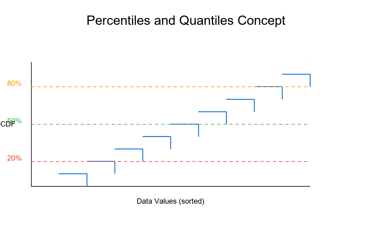
📊 ECDF picture (what to imagine)

• Plot x on the horizontal axis, Fₙ(x) on the vertical (a step function).
• The p‑th percentile is where the ECDF first reaches height p.
  Draw a horizontal line at p, find where it hits the ECDF, drop a vertical line to the x‑axis—that x is the quantile.

Even without a plot, the "sorted list + position" mental model captures the same idea.

🎯 Properties that matter day‑to‑day

• Monotone invariance:
  If you apply a strictly increasing transform f (e.g., converting units, applying exp), the ranks don't change. The quantiles move by exactly f: Q_{f(X)}(p) = f(Q_X(p)).
• Rescaling/shift invariance (with a>0):
  Q_{aX+b}(p) = a·Q_X(p) + b
• Robustness vs outliers:
  One huge outlier shifts the mean, but most quantiles barely move (except the extreme tails).

🚀 Where percentiles are used in Data Science

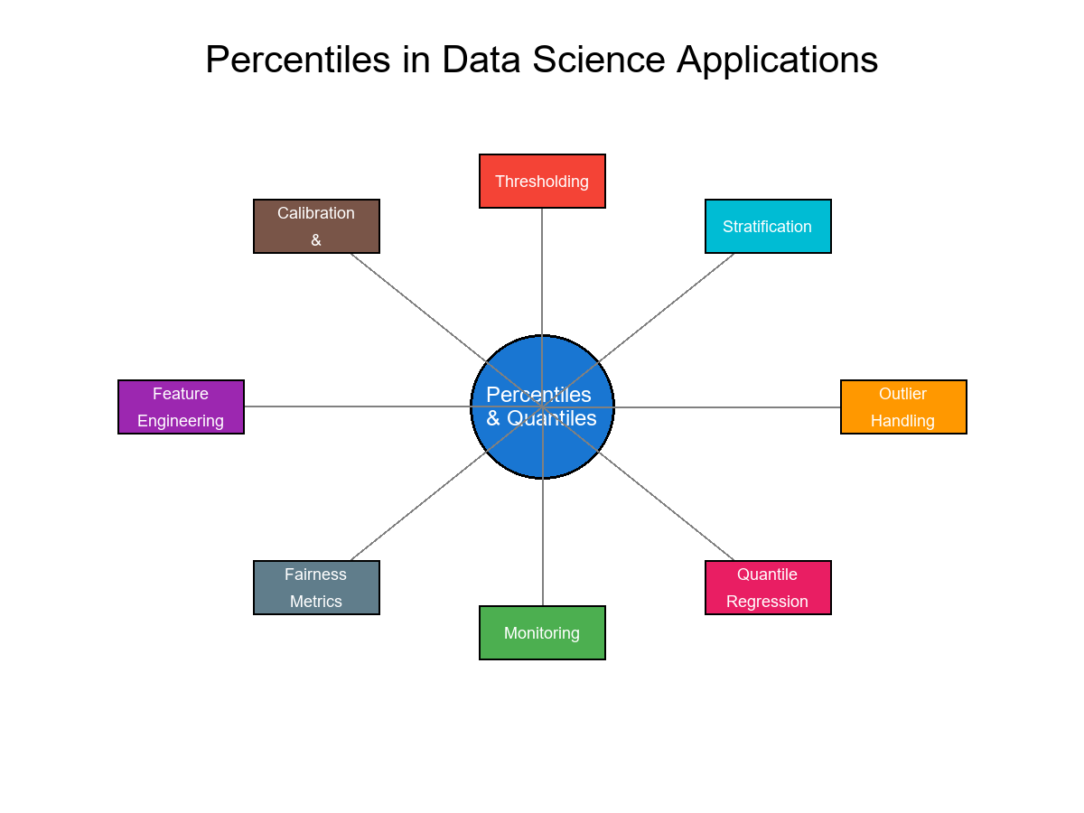
• 🎯 Thresholding: pick cut‑offs at, say, the 95th percentile.
• 👥 Stratification: split a population into deciles/quantile bins.
• 🛡️ Outlier handling: winsorize/clip at given percentiles.
• ⚖️ Calibration bins and fairness audits: compare metrics by quantile slices.
• 📈 Quantile loss models: quantile regression uses the "pinball" loss to estimate Q(p).
• 🔧 Feature engineering: percentile ranks (ECDF values) make features comparable across scales.
• 📊 Monitoring: detect drift by comparing quantiles over time.

🔬 One more worked example — scaling check

Data (sorted): [2, 5, 8, 11, 20]
Take p = 0.6 (60th), using Type 7:

• n = 5; h = 1+(4·0.6) = 3.4; j = 3, γ = 0.4
• Q₀.₆₀ = 0.6·x(3) + 0.4·x(4) = 0.6·8 + 0.4·11 = 4.8 + 4.4 = 9.2

Now rescale: y = 3·x + 2 → transformed data (sorted): [8, 17, 26, 35, 62]
Compute 60th again:

• h same (indices only depend on p and n); use y-values:
  Q_{y,0.6} = 0.6·26 + 0.4·35 = 15.6 + 14 = 29.6

Check invariance:
3·Q₀.₆₀ + 2 = 3·9.2 + 2 = 27.6 + 2 = 29.6 ✔

💡 Practical tips

• ✅ Always state which definition you use (nearest rank, Type 7, etc.).
• 🔍 Handle missing values (drop or impute) before computing percentiles.
• ⚖️ For weighted data, use weighted quantiles (not covered here, but conceptually similar).
• 🤝 For reproducibility in teams, standardize on a single method across code and dashboards.

🌟 Takeaway

Percentiles and quantiles are simple, powerful ways to describe "where" a value sits in the data. They're stable, interpretable, and play well with transformations. Whether you're setting thresholds, creating strata, or monitoring distributions, quantiles give you a clean, math‑first foundation.

📚 References

1. Hyndman, R. J., & Fan, Y. (1996). Sample quantiles in statistical packages. The American Statistician, 50(4), 361-365.

2. Serfling, R. J. (2009). Approximation Theorems of Mathematical Statistics. John Wiley & Sons.

3. Mosteller, F., & Tukey, J. W. (1977). Data Analysis and Regression: A Second Course in Statistics. Addison-Wesley.

4. David, H. A., & Nagaraja, H. N. (2003). Order Statistics (3rd ed.). John Wiley & Sons.

5. Parzen, E. (1979). Nonparametric statistical data modeling. Journal of the American Statistical Association, 74(365), 105-121.

6. Koenker, R. (2005). Quantile Regression. Cambridge University Press.

7. Langford, E. (2006). Quartiles in elementary statistics. Journal of Statistics Education, 14(3).

8. Cramér, H. (1946). Mathematical Methods of Statistics. Princeton University Press.

9. Hoaglin, D. C., Mosteller, F., & Tukey, J. W. (Eds.). (1983). Understanding Robust and Exploratory Data Analysis. John Wiley & Sons.

10. Shorack, G. R., & Wellner, J. A. (2009). Empirical Processes with Applications to Statistics. Society for Industrial and Applied Mathematics.