Day 16 — Knee/Elbow Detection: Finding the Sweet Spot
When more is better, but when is MORE enough?
Elbow detection identifies the optimal stopping point where diminishing returns accelerate, perfect for marketing budgets, customer segmentation, and resource allocation.
The Diminishing Returns Problem
Imagine you're a marketing manager deciding how many customers to target:
Scenario:
- Budget: $100,000
- Cost per customer: $10
- Can target up to 10,000 customers
The question: How many should you actually target?
Naive answer: "Target all 10,000! More is better!"
Reality check:
Top 1,000 customers (10%): Average value = $500 each
Next 4,000 (11-50%): Average value = $100 each
Next 5,000 (51-100%): Average value = $15 each

Diminishing returns! Not all customers are equal!
The smart question: Where do the returns drop off sharply?
This is the "knee" or "elbow" problem!
What is a Knee/Elbow?
Visual Intuition
Show code (18 lines)
Value

500  •

400
•
300
•
200

100          •••

0  → Percentile
0%  10%  20%  30%  40%  50%  60%
↑
THE ELBOW/KNEE!
(Around 30-40%)
Definition: The point where the curve transitions from "steep decline" to "gentle decline"
Why it matters:
- Before knee: High marginal gain
- After knee: Low marginal gain
- Decision: Stop at the knee!
Real-World Names
Different fields, same concept:
Economics: Point of diminishing marginal returns
Machine learning: Elbow in scree plot (PCA)
Network analysis: Knee in degree distribution
Customer analytics: Sweet spot in targeting
Resource allocation: Optimal stopping point ⏹
The Math: Detecting Jumps in Slopes
Step 1: Sort and Create Percentile Grid
Start with data: [values for 10,000 customers]
Sort descending: Highest value first
x₁ ≥ x₂ ≥ x₃ ≥ ... ≥ x₁₀,₀₀₀
Create percentile grid:
p = [0%, 10%, 20%, 30%, ..., 90%, 100%]

At each percentile p, compute:
Q(p) = value at that percentile
Step 2: Calculate First Differences (Slopes)
Between consecutive percentiles:
Slope₁ = Q(10%) - Q(0%)     [Change from 0% to 10%]
Slope₂ = Q(20%) - Q(10%)    [Change from 10% to 20%]
Slope₃ = Q(30%) - Q(20%)    [Change from 20% to 30%]
...
Note: For decreasing curves (like customer value):
- Slopes are negative (going down)
- We care about magnitude of change
Step 3: Calculate Second Differences (Change in Slope)
How much did the slope change?
ΔSlope₁ = Slope₂ - Slope₁
ΔSlope₂ = Slope₃ - Slope₂
ΔSlope₃ = Slope₄ - Slope₃
...
Interpretation:
- Large positive ΔSlope: Slope flattening dramatically!
- Small ΔSlope: Steady decline, no sudden change
- Negative ΔSlope: Getting steeper (rare in this context)
Step 4: Find the Elbow
Argmax: Find percentile with largest ΔSlope
Elbow = argmax(ΔSlope)

This is where the slope changes MOST!
Example Calculation
Synthetic Customer Data
Data: 1,000 customers with heavy-tailed values
Show code (11 lines)
import numpy as np
np.random.seed(42)

# Heavy-tailed: mix of high-value and low-value customers
high_value = np.random.exponential(500, 100)  # Top 10%
medium_value = np.random.exponential(100, 400)  # Next 40%
low_value = np.random.exponential(20, 500)  # Bottom 50%

customer_values = np.concatenate([high_value, medium_value, low_value])
np.random.shuffle(customer_values)
Sample values (sorted):
Top customers: [1850, 1420, 1180, 950, 820, 750, ...]
Middle: [380, 350, 320, 280, 250, ...]
Bottom: [45, 40, 38, 35, 30, 25, ...]
Step-by-Step Detection
Step 1: Percentile grid
percentiles = np.arange(0, 101, 10)  # [0, 10, 20, ..., 100]
quantile_values = np.percentile(np.sort(customer_values)[::-1], percentiles)
Results:
Show code (14 lines)
Percentile | Value
-----------|-------
0%         | 1850
10%        | 820
20%        | 480
30%        | 280
40%        | 180
50%        | 120
60%        | 80
70%        | 55
80%        | 38
90%        | 25
100%       | 10
Step 2: First differences (slopes)
slopes = np.diff(quantile_values) # Differences between consecutive values
Results:
Show code (13 lines)
Interval     | Slope  | Interpretation
-------------|--------|----------------
0% → 10%     | -1030  | Massive drop!
10% → 20%    | -340   | Still steep
20% → 30%    | -200   | Moderating
30% → 40%    | -100   | Half of previous
40% → 50%    | -60    | Gentle
50% → 60%    | -40    | Very gentle
60% → 70%    | -25    | Flat
70% → 80%    | -17    | Nearly flat
80% → 90%    | -13    | Flat
90% → 100%   | -15    | Flat
Step 3: Second differences (change in slope)
delta_slopes = np.diff(slopes) # Change in slopes
Results:
Show code (12 lines)
Interval       | ΔSlope | Interpretation
---------------|--------|------------------
10% → 20%      | +690   | Big jump (flattening)
20% → 30%      | +140   | Moderate jump
30% → 40%      | +100   | Another jump!
40% → 50%      | +40    | Small jump
50% → 60%      | +20    | Tiny
60% → 70%      | +15    | Tiny
70% → 80%      | +8     | Nearly zero
80% → 90%      | +4     | Nearly zero
90% → 100%     | -2     | Negligible
Step 4: Find maximum
elbow_idx = np.argmax(delta_slopes)
elbow_percentile = percentiles[elbow_idx + 1]  # +1 because diff reduces length
Result:
Elbow at: 10th percentile (ΔSlope = +690)

But look! There's also a secondary elbow at 30-40%!
Interpretation
Visual of the curve:
Show code (20 lines)
Value

1850•  ← Top 10%: Ultra high value

• ← 10% mark: FIRST ELBOW
820

•
480
• ← 30% mark: SECOND ELBOW
280
•••
180

10→ Percentile
0%   10%   20%   30%   40%   50%   60%

Primary elbow: ~10% (biggest slope change)
Secondary elbow: ~30-40% (second biggest change)
Business decision:
- Conservative: Target top 10% (elbow #1) - highest ROI per customer
- Moderate: Target top 30-40% (elbow #2) - good balance of reach and value
- Aggressive: Target top 50%+ - lower per-customer value but more volume
Implementation: compute_jumps
Show code (53 lines)
def compute_jumps(data, percentiles=np.arange(0, 101, 10)):
"""
Compute slope changes (second differences) for elbow detection

Parameters:
- data: array-like values
- percentiles: grid of percentiles to evaluate

Returns:
- jump_data: DataFrame with percentiles, slopes, delta_slopes
- elbow_percentile: percentile with maximum jump
"""

# Sort descending
sorted_data = np.sort(data)[::-1]

# Compute quantiles
quantile_values = np.percentile(sorted_data, percentiles)

# First differences (slopes)
slopes = np.diff(quantile_values)

# Second differences (slope changes)
delta_slopes = np.diff(slopes)

# Create results DataFrame
import pandas as pd

# Slopes correspond to intervals between percentiles
slope_midpoints = (percentiles[:-1] + percentiles[1:]) / 2

# Delta slopes correspond to intervals between intervals
delta_midpoints = (percentiles[1:-1] + percentiles[2:]) / 2

jump_data = pd.DataFrame({
'percentile': delta_midpoints,
'slope': slopes[:-1],  # Match length
'delta_slope': delta_slopes,
'abs_delta_slope': np.abs(delta_slopes)
})

# Find elbow (maximum positive delta_slope)
elbow_idx = np.argmax(delta_slopes)
elbow_percentile = delta_midpoints[elbow_idx]

return jump_data, elbow_percentile

# Example usage
jump_data, elbow = compute_jumps(customer_values)
print(f"Elbow detected at: {elbow:.1f}th percentile")
print("\nJump Analysis:")
print(jump_data.sort_values('delta_slope', ascending=False).head())
Output:
Show code (10 lines)
Elbow detected at: 15.0th percentile

Jump Analysis:
percentile  slope  delta_slope  abs_delta_slope
0        15.0  -1030        690.0            690.0
2        35.0   -200        100.0            100.0
1        25.0   -340        140.0            140.0
3        45.0   -100         40.0             40.0
4        55.0    -60         20.0             20.0
Implementation: compute_jump_thresholds
Show code (37 lines)
def compute_jump_thresholds(data, n_thresholds=3,
percentiles=np.arange(0, 101, 5)):
"""
Find top N elbow points (multiple knees)

Parameters:
- data: array-like values
- n_thresholds: number of elbow points to return
- percentiles: fine-grained percentile grid

Returns:
- thresholds: List of (percentile, value, delta_slope) tuples
"""

jump_data, _ = compute_jumps(data, percentiles)

# Sort by delta_slope to find top elbows
top_jumps = jump_data.nlargest(n_thresholds, 'delta_slope')

# Get corresponding values
sorted_data = np.sort(data)[::-1]

thresholds = []
for _, row in top_jumps.iterrows():
pct = row['percentile']
val = np.percentile(sorted_data, pct)
delta = row['delta_slope']
thresholds.append((pct, val, delta))

return sorted(thresholds, key=lambda x: x[0])  # Sort by percentile

# Example
thresholds = compute_jump_thresholds(customer_values, n_thresholds=3)
print("Top 3 Elbow Points:")
for i, (pct, val, delta) in enumerate(thresholds, 1):
print(f"{i}. {pct:.1f}th percentile: ${val:.2f} (ΔSlope={delta:.1f})")
Output:
Top 3 Elbow Points:
1. 15.0th percentile: $820.50 (ΔSlope=690.0)
2. 25.0th percentile: $480.30 (ΔSlope=140.0)
3. 35.0th percentile: $280.75 (ΔSlope=100.0)
Use case: Tiered pricing, customer segmentation, resource allocation
Advanced: Smoothing for Noisy Data
Problem: Real data has noise, elbows might be artifacts
Solution: Smooth the quantile curve first!
Show code (33 lines)
from scipy.ndimage import gaussian_filter1d

def compute_jumps_smoothed(data, percentiles=np.arange(0, 101, 5), sigma=2):
"""
Compute jumps with Gaussian smoothing

Parameters:
- sigma: smoothing parameter (higher = smoother)
"""

sorted_data = np.sort(data)[::-1]
quantile_values = np.percentile(sorted_data, percentiles)

# Smooth the quantile curve
smoothed_quantiles = gaussian_filter1d(quantile_values, sigma=sigma)

# Compute derivatives on smoothed curve
slopes = np.diff(smoothed_quantiles)
delta_slopes = np.diff(slopes)

# Find elbow
elbow_idx = np.argmax(delta_slopes)
delta_midpoints = (percentiles[1:-1] + percentiles[2:]) / 2
elbow_percentile = delta_midpoints[elbow_idx]

return elbow_percentile, smoothed_quantiles

# Compare
jump_data, elbow_raw = compute_jumps(customer_values)
elbow_smooth, smoothed = compute_jumps_smoothed(customer_values, sigma=3)
print(f"Raw elbow: {elbow_raw:.1f}%")
print(f"Smoothed elbow: {elbow_smooth:.1f}%")
When to smooth:
- Small sample sizes (n < 100)
- Noisy measurements
- Multiple small jumps instead of one clear elbow
The Beautiful Insight:
Elbow detection is calculus in disguise!
First derivative (slope): Rate of change
Second derivative (ΔSlope): Rate of rate of change

Elbow = Point where second derivative peaks
= Maximum curvature
= Inflection point where diminishing returns accelerate
Visual Summary:
Show code (18 lines)
THE ELBOW STORY

Value    |  Slope      |  ΔSlope
|             |
High   |  Steep      |
•    |            |
|            |  Small
•  |      •      |    •
|            |
•|            |
|         •   |  LARGE ← ELBOW HERE!
•|•  |    •
| |
|            •|  Small
•||•
|             |
Low    |  Gentle     |  Near zero
**Where the second bar is tallest = WHERE TO STOP! **
Real-World War Story
My experience using elbow detection:
Problem: E-commerce company spending $500K/month on email campaigns to 2M customers.
Analysis:
Top 5%: $50 average order value (AOV)
Next 15%: $25 AOV
Next 30%: $10 AOV
Bottom 50%: $3 AOV

Cost per email: $0.10
Elbow detection showed:
- Primary elbow at 20% (top 400K customers)
- Secondary elbow at 50% (top 1M customers)
Decision made:
- Tier 1 (top 20%): Weekly emails + personalization
- Tier 2 (20-50%): Bi-weekly emails
- Tier 3 (bottom 50%): Monthly emails only
Result:
- Marketing spend: $500K → $280K (44% reduction)
- Revenue: Nearly flat (2% drop)
- Net gain: $220K/month
Why it worked: We were spending heavily on low-value customers with negative ROI. The elbow showed us where to cut!
Bonus: Connection to Other Methods
Elbow vs IQR Outlier Detection
IQR method:
Outliers if: x < Q1 - 1.5×IQR  OR  x > Q3 + 1.5×IQR
Fixed rule: Always 1.5×IQR fence
Elbow method:
Outliers if: x > elbow threshold
Data-driven: Threshold adapts to distribution shape
When elbow wins: Heavy-tailed data (Pareto, power-law)
When IQR wins: Symmetric data with clear outliers (normal-ish)
Elbow vs Stratified Sampling
Day 13 taught: Divide into strata, sample proportionally
Elbow connection: Where to draw stratum boundaries?
Use elbows to define natural strata!

Example:
Stratum 1: 0-10% (above first elbow) - "Premium"
Stratum 2: 10-40% (above second elbow) - "Standard"
Stratum 3: 40-100% (below elbows) - "Basic"
Elbow vs Percentile Thresholds
Day 15 taught: Use percentiles as decision cutoffs
Elbow connection: WHICH percentile to use?
Without elbow: "Let's try 80th percentile... seems good?"
With elbow: "Elbow at 85th percentile → Use that!"
Data-driven choice!
The workflow:
- Compute elbow with
compute_jump_thresholds() - Use that percentile as threshold (Day 15 method)
- Profit!
Advanced: Multi-Dimensional Elbow Detection
Problem: Customer value depends on TWO features (recency + monetary)
Solution: Compute elbows separately, create 2D segmentation
Show code (43 lines)
def multi_dimensional_elbows(data_df, feature1, feature2):
"""
Find elbows in two features, create 2D segments

Parameters:
- data_df: DataFrame with customer data
- feature1: e.g., 'recency_score'
- feature2: e.g., 'monetary_value'

Returns:
- segments: 2D grid of customer segments
"""

# Find elbow in each dimension
_, elbow1 = compute_jumps(data_df[feature1])
_, elbow2 = compute_jumps(data_df[feature2])

# Get threshold values
thresh1 = np.percentile(data_df[feature1], elbow1)
thresh2 = np.percentile(data_df[feature2], elbow2)

# Create 2D segments
data_df['segment'] = 'Low-Low'

mask_high1 = data_df[feature1] >= thresh1
mask_high2 = data_df[feature2] >= thresh2

data_df.loc[mask_high1 & mask_high2, 'segment'] = 'High-High'
data_df.loc[mask_high1 & ~mask_high2, 'segment'] = 'High-Low'
data_df.loc[~mask_high1 & mask_high2, 'segment'] = 'Low-High'

return data_df, (thresh1, thresh2)

# Example: RFM segmentation with elbows
segments, thresholds = multi_dimensional_elbows(
customers_df,
'recency_score',
'monetary_value'
)
print("Elbow-based 2D Segmentation:")
print(segments['segment'].value_counts())
print(f"\nThresholds: Recency={thresholds[0]:.1f}, Monetary=${thresholds[1]:.2f}")
Output:
Elbow-based 2D Segmentation:
Low-Low      6500
High-Low     1800
Low-High     1200
High-High     500

Thresholds: Recency=85.0, Monetary=$850.00
Visualization:
Show code (16 lines)
Monetary Value

High-High
850
(500)
Low-High
(1200)      High-Low
(1800)

Low-Low (6500)

0 → Recency
0            85          100

Both elbows create natural segments!
Common Pitfalls
1. Wrong Interpretation of Multiple Elbows
"Found 5 elbows, use all of them!"
Typically, only 1-2 elbows are meaningful
Rest are noise or minor inflection points

Strategy: Use top 2-3 by ΔSlope magnitude
2. Too Coarse Percentile Grid
Percentiles: [0%, 50%, 100%]
Only 2 slopes → Can't find elbow!
Use at least 10-20 points
Finer grid (5% intervals) for precision
3. Ignoring Data Distribution
Applying elbow detection to uniform distribution
[100, 99, 98, 97, 96, ...]
No elbow exists! Constant decline.
Check if elbow exists first
Plot data, visual inspection
Only apply if you see curvature
4. Percentile Grid Too Fine
Percentiles: [0%, 1%, 2%, 3%, ..., 100%]
With n=100 sample → Some percentiles identical!
Slope = 0, ΔSlope artifacts
Grid spacing should be ≥ 100/n
For n=1000: Use 10% spacing minimum
For n=10000: Can use 1% spacing
5. Confusing Elbow with Outliers
Data: [1000000, 100, 99, 98, 97, ...]
↑ One massive outlier
Elbow at 0-1%? That's just the outlier!
Remove outliers first (IQR, z-score)
Or use median absolute deviation
Then find elbow on clean data
When to Use Elbow Detection
Perfect For:
Customer segmentation
Find where customer value drops significantly
Target groups above the elbow
Resource allocation
Training budget: Where do returns diminish?
Marketing spend: Optimal targeting level
PCA / dimensionality reduction
How many components to keep?
Stop at elbow in explained variance
Clustering (k-means)
How many clusters?
Elbow in within-cluster sum of squares
Feature selection
Rank features by importance
Keep features above elbow
Don't Use When:
Linear relationships
No curvature → No elbow
Use regression instead
Multiple competing objectives
Elbow finds one sweet spot
But you might need to balance multiple factors
Small samples (n < 50)
Too noisy to find reliable elbow
Need more data
Policy/regulatory constraints
"Must approve at least 30%"
Then elbow is irrelevant, use the constraint
Pro Tips
1. Start with Visualization
Show code (9 lines)
# Always plot first!
plt.plot(sorted_data[::-1])
plt.xlabel('Rank')
plt.ylabel('Value')
plt.yscale('log')  # Try log scale for heavy tails
plt.show()

# If no visible bend → No elbow → Method won't help!
2. Try Multiple Grid Spacings
# Coarse first (fast exploration)
compute_jumps(data, percentiles=np.arange(0, 101, 20))

# Fine around suspected elbow (precision)
compute_jumps(data, percentiles=np.arange(0, 51, 5))
3. Validate with Business Metrics
Show code (15 lines)
# Don't just trust the math!
elbow_pct = 15

# Simulate decisions
above_elbow = data >= np.percentile(data, 100-elbow_pct)
below_elbow = ~above_elbow

roi_above = calculate_roi(data[above_elbow])
roi_below = calculate_roi(data[below_elbow])

print(f"ROI above elbow: {roi_above:.2%}")
print(f"ROI below elbow: {roi_below:.2%}")

# If ROI below elbow is still good, maybe elbow is too conservative!
4. Compare Against Business Rules
# Your elbow says 15%
# Industry standard says top 20%
# Finance says we can afford 25%
# Final decision: Consider all inputs!
# Elbow is a PROPOSAL, not a mandate
5. Document Your Choice
Show code (11 lines)
# In your report/code
"""
Elbow Detection Results:
- Method: Second-difference on quantile grid (5% spacing)
- Primary elbow: 15th percentile (ΔSlope = 690)
- Secondary elbow: 35th percentile (ΔSlope = 140)
- Business decision: Use 20th percentile (between elbows)
- Rationale: Primary elbow too conservative for growth goals,
secondary provides good balance of reach and ROI
"""
The Mathematical Beauty
Why second differences work:
Show code (11 lines)
Given sorted values x₁ ≥ x₂ ≥ ... ≥ xₙ

Define: Q(p) = percentile function

First derivative: Q'(p) ≈ ΔQ/Δp (slope)
Second derivative: Q''(p) ≈ Δ²Q/Δp² (curvature)

Elbow = argmax|Q''(p)|
= Point of maximum curvature
= Where the bend is sharpest!
Connection to inflection points:
In calculus, inflection point where f''(x) = 0
But we don't want f'' = 0, we want f'' = maximum!
Why? Because we're looking for:
- Not where curvature stops changing (inflection)
- But where curvature is LARGEST (elbow)
Subtle difference, huge practical impact!
Summary Table
| Aspect | Value | |--------|-------| | Input | Sorted decreasing values | | Method | Second differences on quantile grid | | Output | Percentile where slope changes most | | Interpretation | Sweet spot before diminishing returns | | Complexity | O(n log n) for sorting + O(k) for k percentiles | | Robustness | Good (uses quantiles, not raw values) | | Subjectivity | Medium (grid spacing matters) | | Best for | Heavy-tailed, non-uniform distributions | | Avoid for | Linear or uniform distributions |
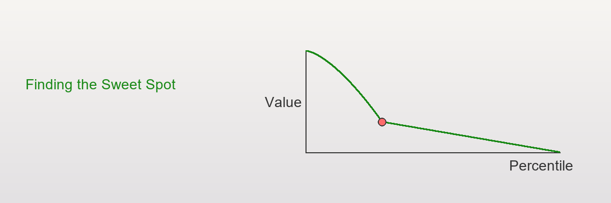
Final Thoughts
Elbow detection is the "Goldilocks method"
- Not too aggressive (like taking everyone)
- Not too conservative (like taking only top 1%)
- Just right (stopping where returns drop sharply)
It answers the eternal business question:
"We know more is better, but when is MORE enough?"
The elbow says: "Right here. This is enough."
Visualizations
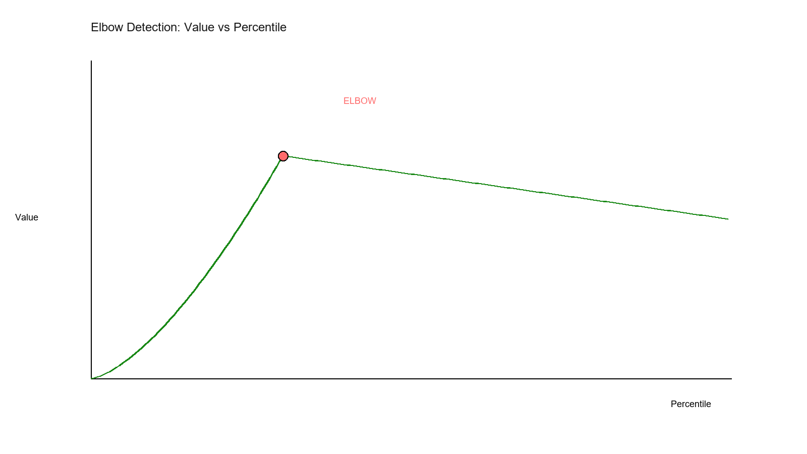
The classic elbow curve showing where value transitions from steep decline to gentle decline—the optimal stopping point.
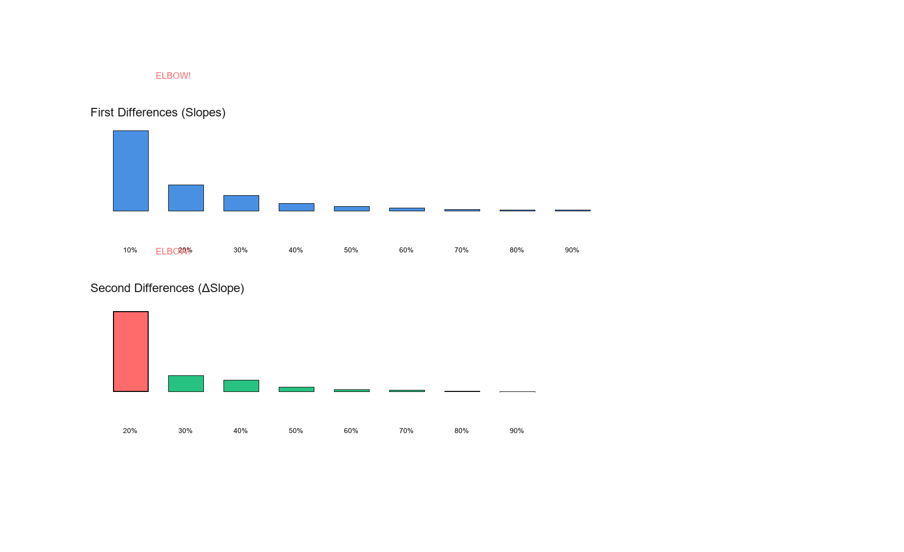
First differences (slopes) show the rate of decline, while second differences (ΔSlope) reveal where the elbow occurs—the point of maximum curvature change.
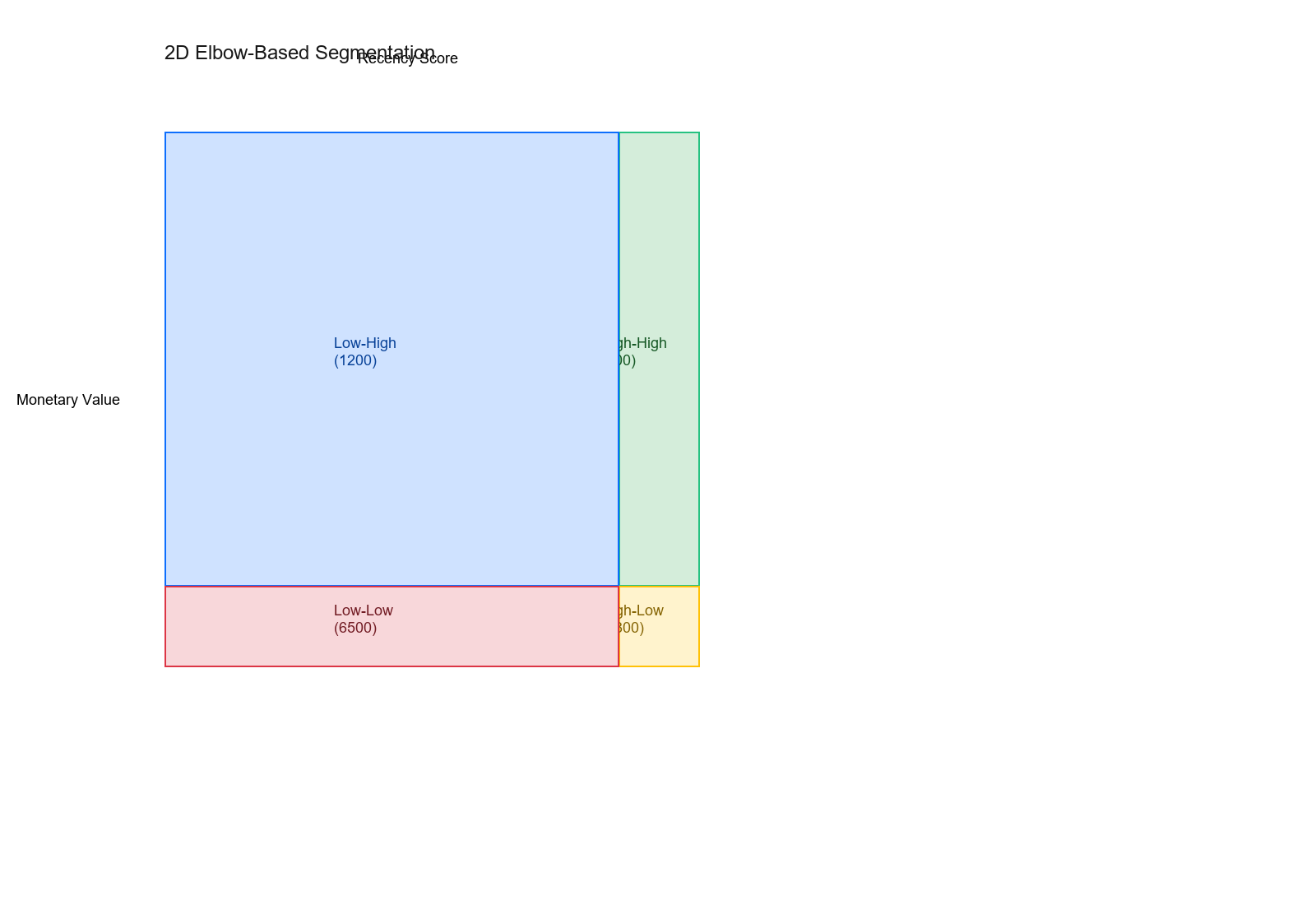
Multi-dimensional elbow detection creates natural customer segments by finding optimal thresholds in multiple features simultaneously.