Day 5 — Robust Location and Scale: Median & MAD (Simple Guide + Worked Example)
Introduction
When data contains outliers, traditional measures like mean and SD can be misleading. Robust statistics like the median and MAD provide stable estimates that resist distortion from extreme values.
In a nutshell:
The mean and standard deviation (SD) can be swayed by outliers like reeds in the wind — a single extreme value can pull them off course.
The median and MAD (Median Absolute Deviation), on the other hand, are sturdy rocks in the statistical stream.
They resist distortion and give reliable "center" and "spread" estimates, even when your data are skewed or heavy-tailed.
Use them to compute robust z-scores, which catch anomalies without being fooled by outliers.
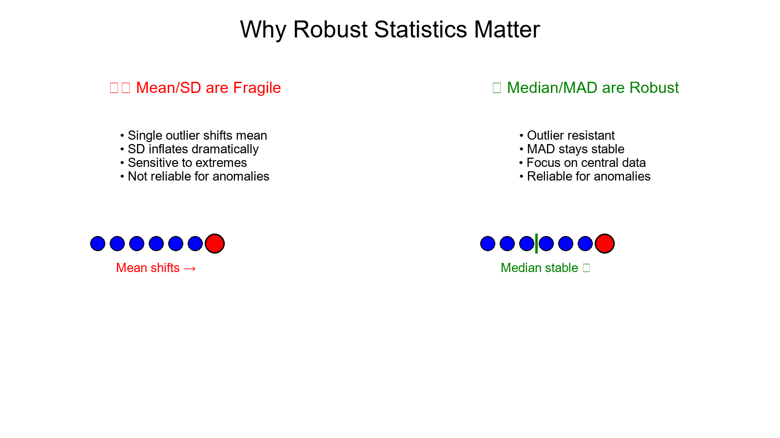
Why Robust Statistics?
Mean/SD are fragile: a single large value can shift both.
Median/MAD are robust: they focus on the central tendency and typical deviation.
Robust z-scores highlight genuine outliers even when your data contain a few extremes.
Key Definitions
Median: the "middle" value after sorting your data (half below, half above).
MAD (Median Absolute Deviation):
- Compute the median m.
- Take absolute deviations |xᵢ − m|.
- Take the median of those deviations → that's MAD.
Robust z-score:
zᵣ = 0.6745 × (x − median) / MAD
Why 0.6745? Because for a Normal distribution, MAD ≈ 0.6745 × SD.
That scaling ensures robust z-scores align roughly with classical z-scores.

Worked Example — Step by Step
Data with one big outlier:
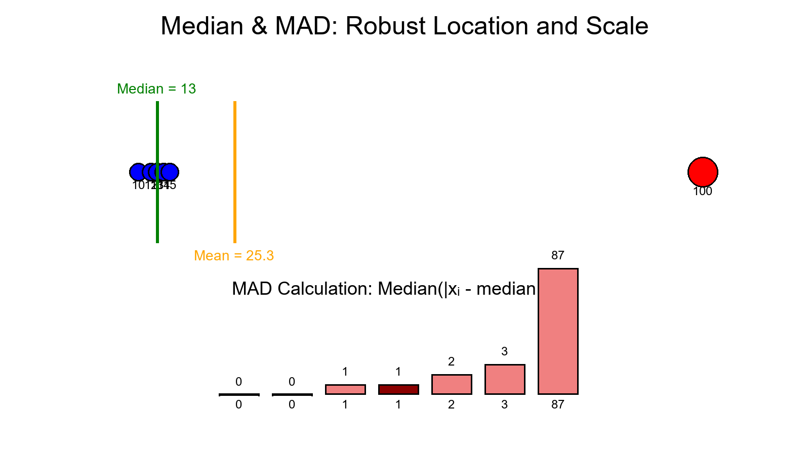
[10, 12, 13, 13, 14, 15, 100]
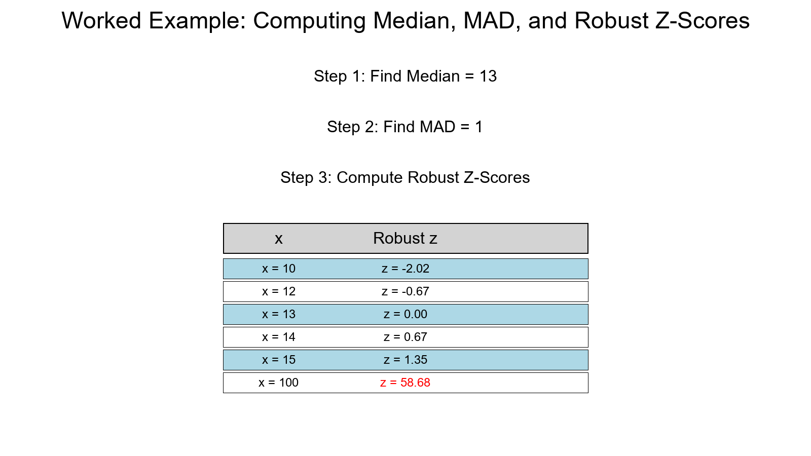
Step 1. — Median
n = 7 → 4th value = 13
Step 2. — Absolute deviations from the median
| x | |x − 13| |
|---|---|
| 10 | 3 |
| 12 | 1 |
| 13 | 0 |
| 13 | 0 |
| 14 | 1 |
| 15 | 2 |
| 100 | 87 |
Sorted deviations: [0, 0, 1, 1, 2, 3, 87]
→ MAD = 1 (the 4th value)
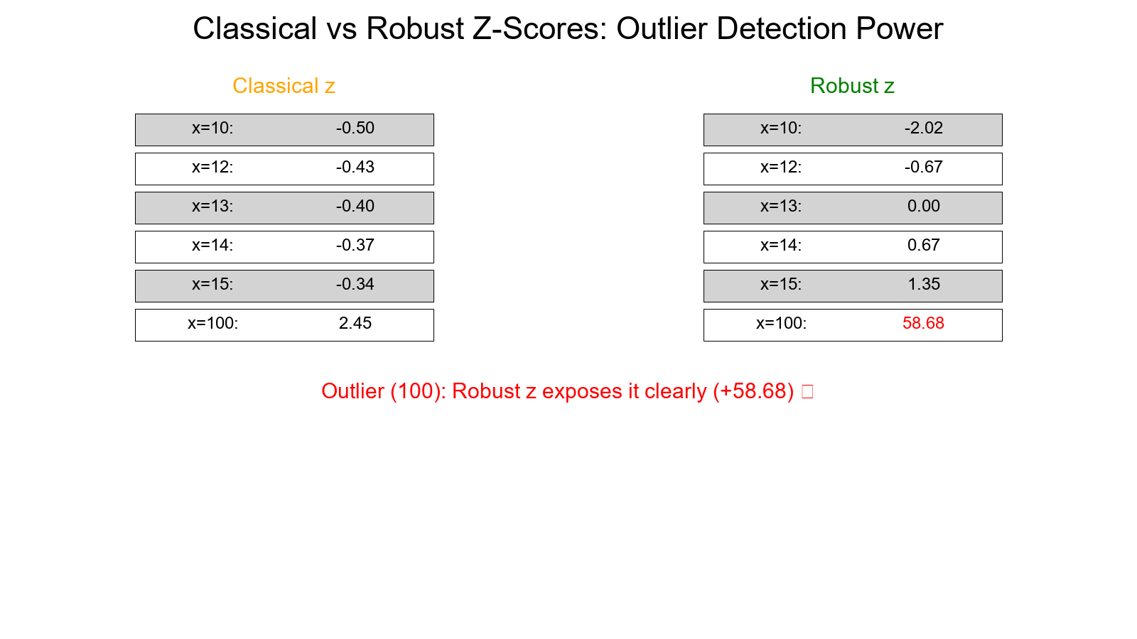
Step 3. — Robust z-scores
zᵣ = 0.6745 × (x − 13) / 1
| x | zᵣ |
|---|---|
| 10 | −2.02 |
| 12 | −0.67 |
| 13 | 0.00 |
| 14 | +0.67 |
| 15 | +1.35 |
| 100 | +58.68 |
Interpretation:
- Most points sit around ±2 — normal variation.
- The outlier (100) explodes to +58.7 — unmistakably extreme.
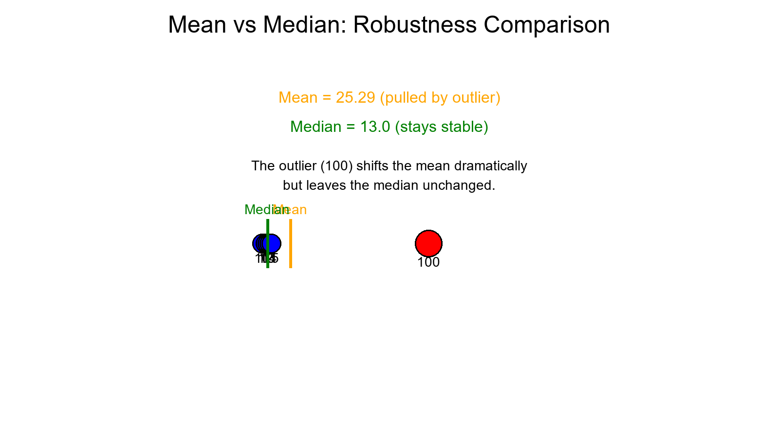
Compare with Mean & SD
Let's see how classical stats behave on the same data:
- Mean ≈ 25.29
- SD ≈ 30.54
Classical z-score for x = 100:
(100 − 25.29) / 30.54 ≈ +2.45
Observation:
- The classical z-score barely flags 100 as unusual (+2.45).
- The robust z-score screams "outlier!" (+58.68).
That's the power of robust measures: they don't let one big number distort the story.
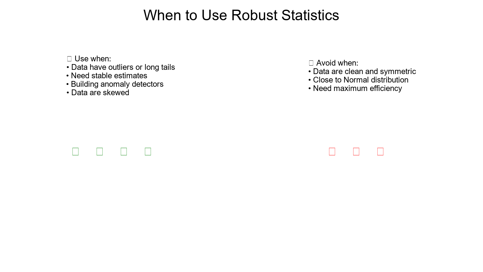
When to Use Median/MAD
Use when:
- Your data have outliers or long tails.
- You need stable estimates of center/spread.
- You're building anomaly detectors or control charts that must resist distortion.
Avoid when:
- Data are clean, symmetric, and close to Normal — mean/SD are slightly more efficient there.
Quick Recipe (Ready to Copy)
-
Sort your data → compute median.
-
Compute absolute deviations → find MAD.
-
Compute for each x:
z_robust = 0.6745 × (x − median) / MAD
- Flag outliers if |zᵣₒbᵤₛₜ| > threshold (common thresholds: 3.5 or 4.5).
Simple. Explainable. Powerful.
Visual Idea (Optional Plot)
Create a scatterplot of classical z vs robust z.
On skewed data, classical z flattens the extremes, while robust z exposes them.
A picture that says a thousand outliers.
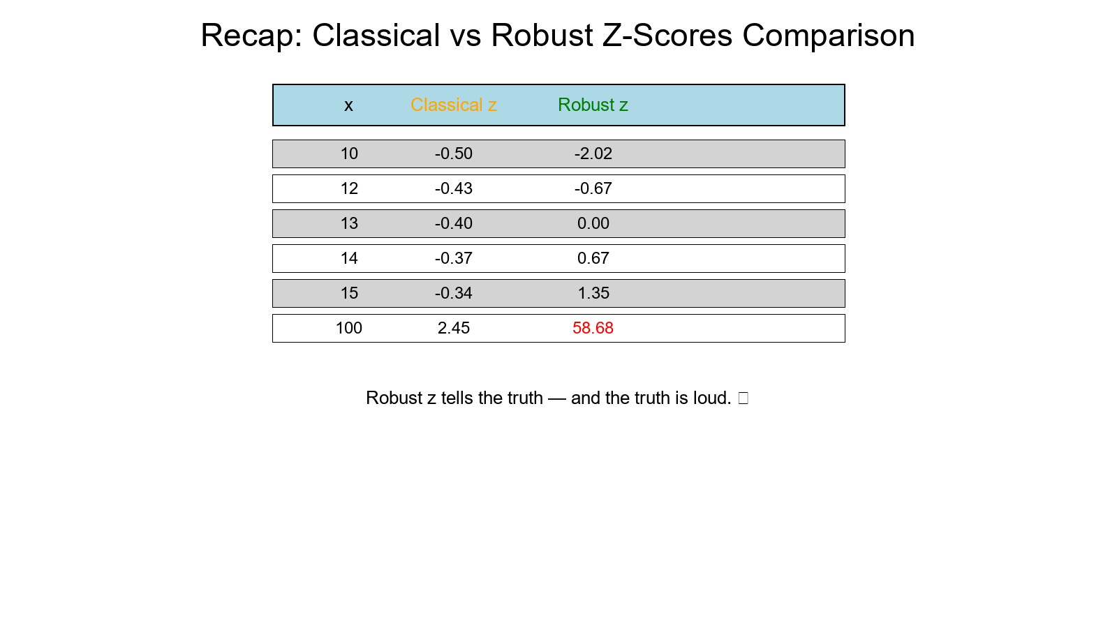
Tiny Recap Table
| x | Classical z | Robust z |
|---|---|---|
| 10 | −0.50 | −2.02 |
| 12 | −0.43 | −0.67 |
| 13 | −0.40 | 0.00 |
| 14 | −0.37 | +0.67 |
| 15 | −0.34 | +1.35 |
| 100 | +2.45 | +58.68 |
Robust z tells the truth — and the truth is loud.
Wrapping Up
- Median + MAD = the sturdier cousins of mean/SD.
- They stay centered when outliers appear.
- Robust z-scores reveal what classical z-scores often hide.
- Use them when your data aren't "nice and Normal."
They'll never overreact — or underreact — to the wild ones.
References
-
Hampel, F. R., Ronchetti, E. M., Rousseeuw, P. J., & Stahel, W. A. (2011). Robust Statistics: The Approach Based on Influence Functions. John Wiley & Sons.
-
Huber, P. J., & Ronchetti, E. M. (2009). Robust Statistics (2nd ed.). John Wiley & Sons.
-
Rousseeuw, P. J., & Croux, C. (1993). Alternatives to the median absolute deviation. Journal of the American Statistical Association, 88(424), 1273-1283.
-
Leys, C., Ley, C., Klein, O., Bernard, P., & Licata, L. (2013). Detecting outliers: Do not use standard deviation around the mean, use absolute deviation around the median. Journal of Experimental Social Psychology, 49(4), 764-766.
-
Mosteller, F., & Tukey, J. W. (1977). Data Analysis and Regression: A Second Course in Statistics. Addison-Wesley.
-
Hoaglin, D. C., Mosteller, F., & Tukey, J. W. (Eds.). (1983). Understanding Robust and Exploratory Data Analysis. John Wiley & Sons.
-
Wilcox, R. R. (2012). Introduction to Robust Estimation and Hypothesis Testing (3rd ed.). Academic Press.
-
Maronna, R. A., Martin, R. D., & Yohai, V. J. (2019). Robust Statistics: Theory and Methods (2nd ed.). John Wiley & Sons.