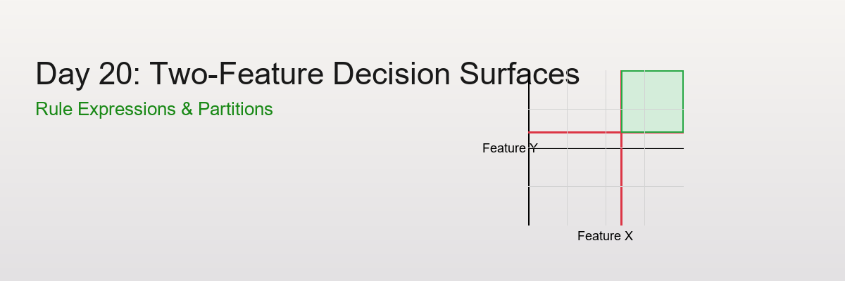
Day 20: Two-Feature Decision Surfaces from Rule Expressions
The Power of Visualizing Rules
Scenario: You're building a risk scoring system with two features:
- Feature X: Transaction amount
- Feature Y: Account age
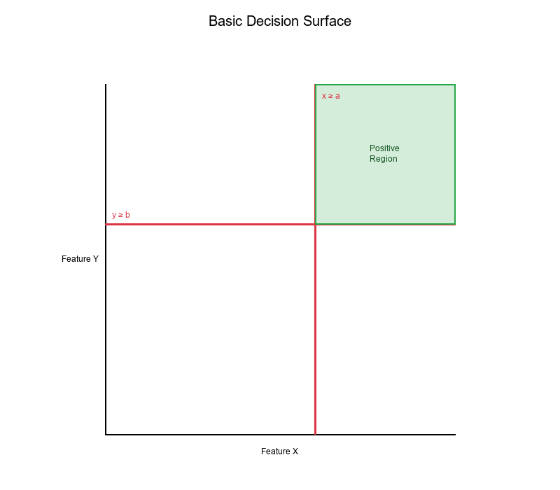
Rule: IF (amount ≥ $1000) AND (age ≥ 30 days) THEN High Risk
Question: What does this rule look like in feature space?
Answer: A rectangular region! The rule creates a decision surface that partitions the 2D space into "High Risk" and "Low Risk" regions.
Visual Example:
Half-Spaces: The Building Blocks
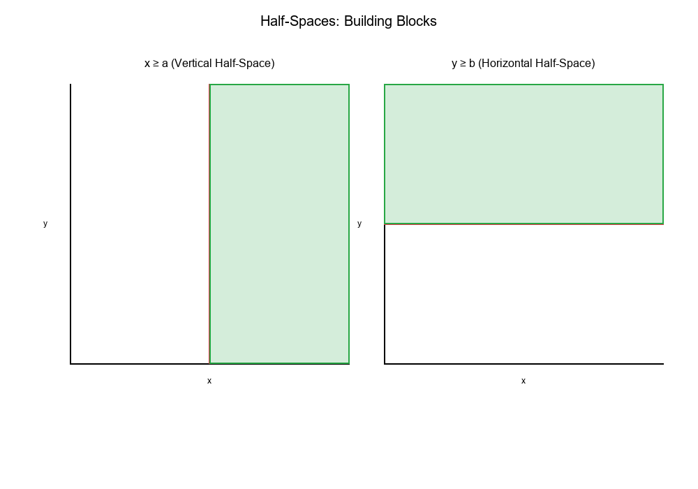
What is a Half-Space?
A half-space is the region on one side of a line (in 2D) or plane (in 3D).
In 2D:
x ≥ acreates a vertical half-space (everything to the right of x = a)y ≥ bcreates a horizontal half-space (everything above y = b)
Visual Example:
Combining Half-Spaces
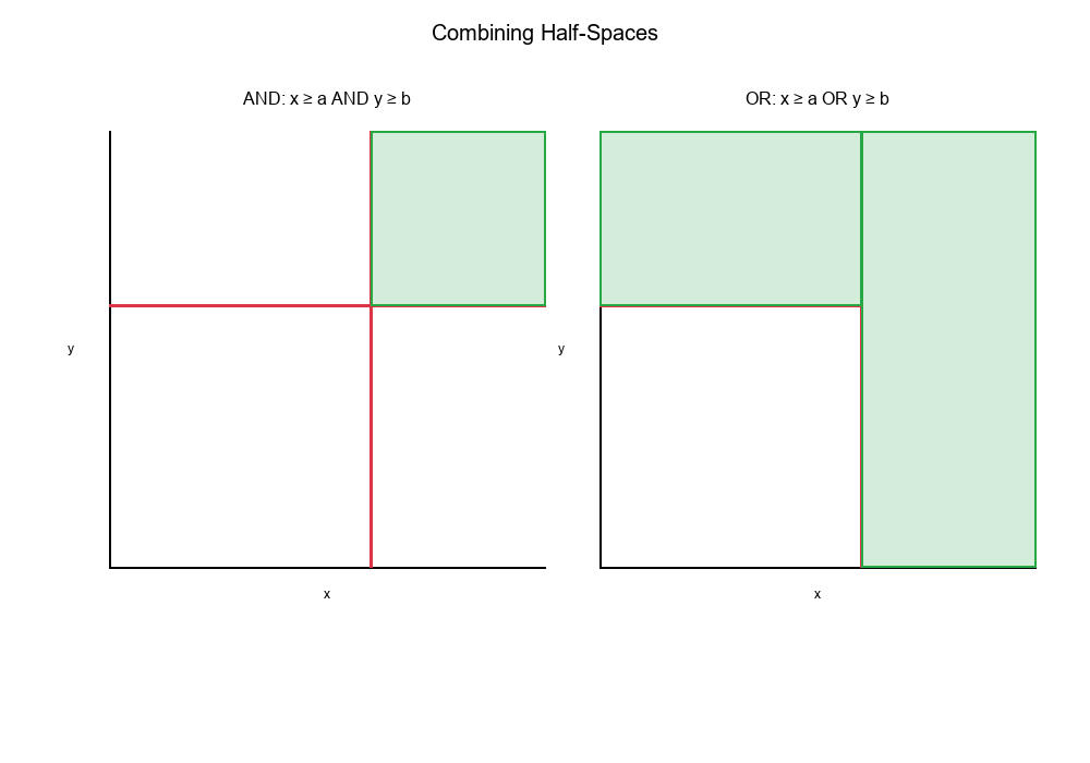
When you combine half-spaces with AND or OR logic, you create more complex regions:
AND (Intersection):
Rule: x ≥ a AND y ≥ b
Result: The intersection of two half-spaces
→ A rectangular region (quadrant)
OR (Union):
Rule: x ≥ a OR y ≥ b
Result: The union of two half-spaces
→ An L-shaped region
Visual Example:
Orthogonal Cut Lines: Creating Quadrants
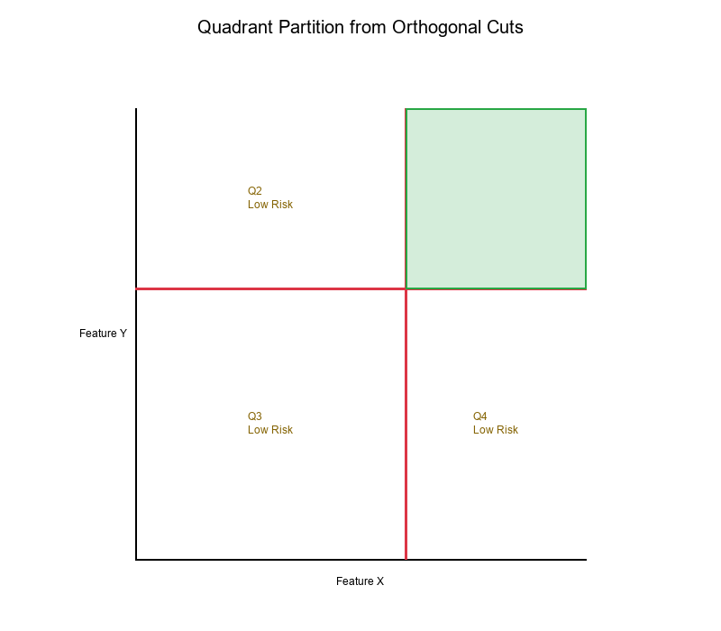
What are Orthogonal Cut Lines?
Orthogonal cut lines are perpendicular lines that divide feature space into regions. In 2D, they're typically:
- Vertical lines:
x = threshold_x - Horizontal lines:
y = threshold_y
Example:
Thresholds:
- x_threshold = 1000
- y_threshold = 30

Cut lines:
- Vertical: x = 1000
- Horizontal: y = 30
Result: Four quadrants:
- Q1 (Top-Right): x ≥ 1000 AND y ≥ 30 → High Risk
- Q2 (Top-Left): x < 1000 AND y ≥ 30 → Low Risk
- Q3 (Bottom-Left): x < 1000 AND y < 30 → Low Risk
- Q4 (Bottom-Right): x ≥ 1000 AND y < 30 → Low Risk
Visual Example:
Decision Surfaces from Rule Expressions
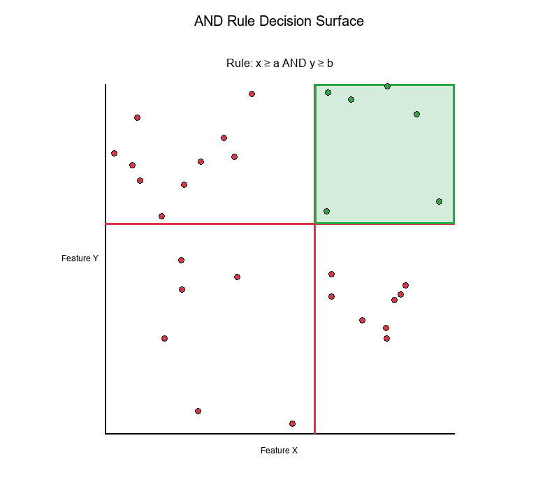
Simple AND Rule
Rule: IF (x ≥ a) AND (y ≥ b) THEN Positive
Decision Surface:
- Creates a rectangular region in the top-right quadrant
- All points in this region are classified as "Positive"
- All other points are classified as "Negative"
Visual Example:
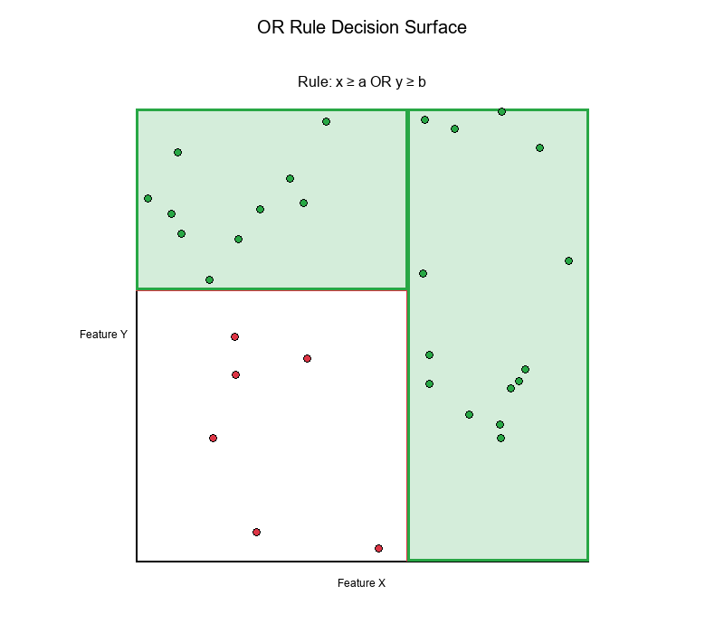
Simple OR Rule
Rule: IF (x ≥ a) OR (y ≥ b) THEN Positive
Decision Surface:
- Creates an L-shaped region
- Covers three quadrants (top-right, top-left, bottom-right)
- Only bottom-left quadrant is "Negative"
Visual Example:
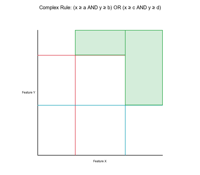
Complex Rules
Rule: IF (x ≥ a AND y ≥ b) OR (x ≥ c AND y ≥ d) THEN Positive
Decision Surface:
- Creates multiple rectangular regions
- Union of two rectangular regions
- More complex partition of feature space
Visual Example:
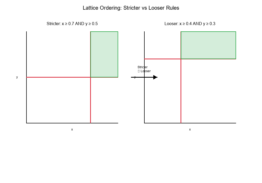
Lattice Ordering: Understanding Threshold Relationships
Connection to Day 1: Lattice ordering helps us understand how threshold changes affect decision surfaces.
What is Lattice Ordering?
In a lattice, we can compare rules based on their "strictness":
- Rule A is stricter than Rule B if Rule A's region is a subset of Rule B's region
- Rule A is looser than Rule B if Rule A's region is a superset of Rule B's region
Example:
Rule 1: x ≥ 1000 AND y ≥ 30  (stricter)
Rule 2: x ≥ 500 AND y ≥ 20   (looser)

Rule 1's region is inside Rule 2's region
→ Rule 1 is stricter than Rule 2
Visual Example:
Threshold Changes and Lattice Ordering
Increasing a threshold makes the rule stricter:
- The decision region shrinks
- Fewer points are classified as positive
- Higher precision, lower recall
Decreasing a threshold makes the rule looser:
- The decision region expands
- More points are classified as positive
- Lower precision, higher recall
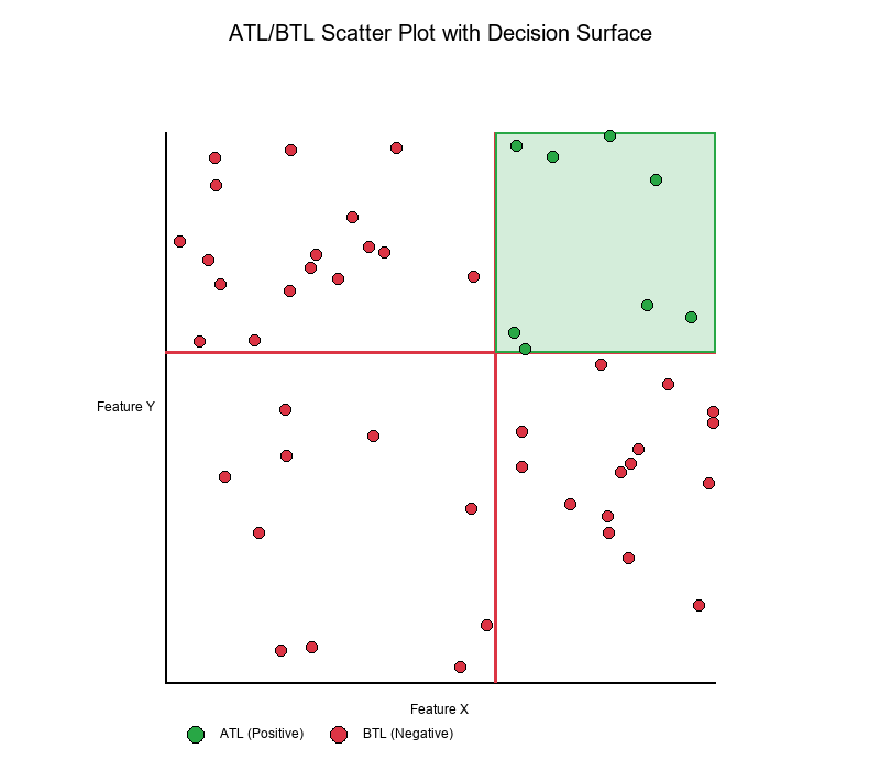
Real-World Application: ATL/BTL Shading
What is ATL/BTL?
ATL (Above The Line): Points that satisfy the rule (classified as positive) BTL (Below The Line): Points that don't satisfy the rule (classified as negative)
create_scatter_plot Function
The create_scatter_plot function visualizes decision surfaces by:
- Plotting data points in 2D feature space
- Drawing threshold lines (cut lines)
- Shading regions based on rule satisfaction
- Color-coding points as ATL (positive) or BTL (negative)
Visual Example:
Code Concept:
Show code (14 lines)
def create_scatter_plot(x_data, y_data, x_threshold, y_threshold, rule_type='AND'):
"""
Create scatter plot with decision surface shading

Parameters:
- x_data, y_data: Feature values
- x_threshold, y_threshold: Rule thresholds
- rule_type: 'AND' or 'OR'
"""
# Plot data points
# Draw threshold lines
# Shade regions based on rule
# Color-code ATL vs BTL points
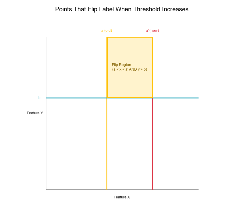
Exercise: Characterizing Points That Flip Labels
The Problem
Question: When you increase threshold a (for feature x), which points flip from "Positive" to "Negative"?
Setup:
Original rule: IF (x ≥ a) AND (y ≥ b) THEN Positive
New rule:      IF (x ≥ a') AND (y ≥ b) THEN Positive
Where: a' > a (threshold increased)
Solution
Points that flip label:
- Must satisfy:
a ≤ x < a'(between old and new threshold) - Must satisfy:
y ≥ b(still above y threshold) - Region: A horizontal strip between the two vertical lines
Visual Example:
Mathematical Characterization
Points that flip from Positive → Negative:
Region: { (x, y) | a ≤ x < a' AND y ≥ b }
Points that flip from Negative → Positive:
None! (Increasing threshold only removes points, never adds)
Key Insight:
- Only points in the "removed strip" flip labels
- The strip is bounded by:
- Left:
x = a(old threshold) - Right:
x = a'(new threshold) - Bottom:
y = b(y threshold) - Top: Infinity
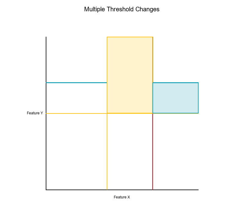
General Case: Changing Multiple Thresholds
Question: What happens when you change both thresholds?
Case 1: Increase both thresholds
Old: x ≥ a AND y ≥ b
New: x ≥ a' AND y ≥ b'  (where a' > a, b' > b)

Points that flip: Region shrinks
- Removed: { (x, y) | (a ≤ x < a' AND y ≥ b) OR (x ≥ a' AND b ≤ y < b') }
Case 2: Increase one, decrease the other
Old: x ≥ a AND y ≥ b
New: x ≥ a' AND y ≥ b'  (where a' > a, b' < b)

Points that flip:
- Lost: { (x, y) | a ≤ x < a' AND y ≥ b }
- Gained: { (x, y) | x ≥ a' AND b' ≤ y < b }
Visual Example:
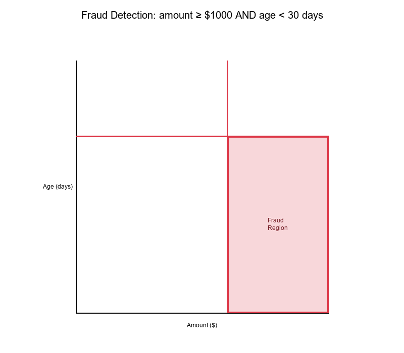
Visualizing Decision Surfaces: Practical Examples
Example 1: Fraud Detection
Features:
- X: Transaction amount ($)
- Y: Account age (days)
Rule: IF (amount ≥ $1000) AND (age < 30 days) THEN Fraud
Decision Surface:
- High-risk region: Bottom-right quadrant
- Low-risk region: All other quadrants
Visual Example:
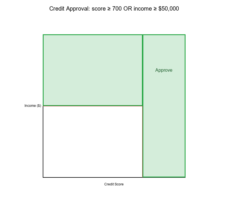
Example 2: Credit Approval
Features:
- X: Credit score
- Y: Income ($)
Rule: IF (score ≥ 700) OR (income ≥ $50,000) THEN Approve
Decision Surface:
- Approval region: L-shaped (three quadrants)
- Rejection region: Bottom-left quadrant only
Visual Example:
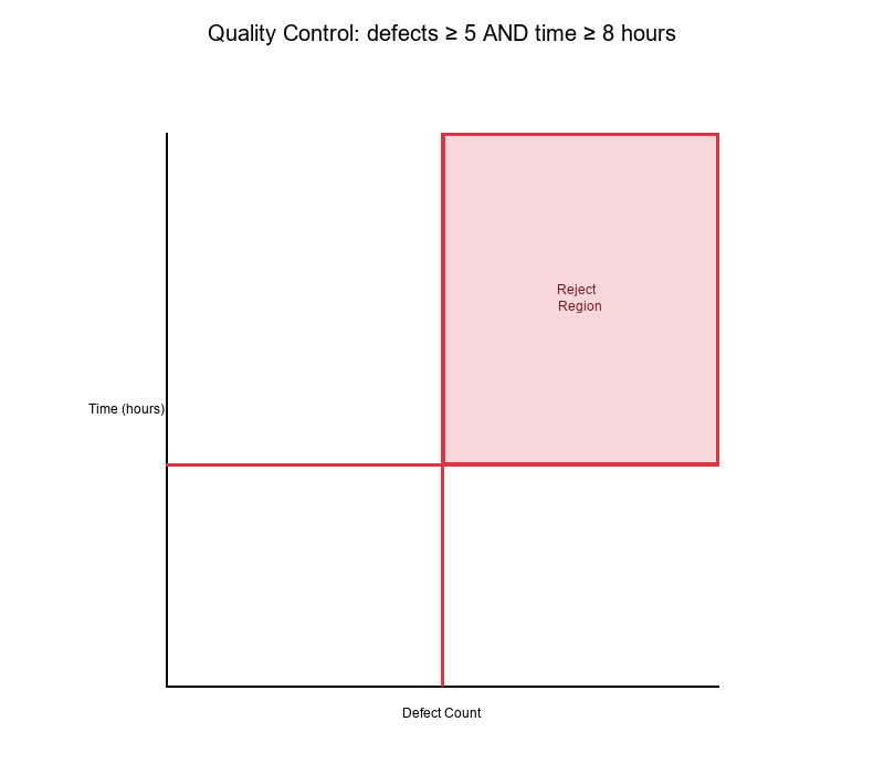
Example 3: Quality Control
Features:
- X: Defect count
- Y: Production time (hours)
Rule: IF (defects ≥ 5) AND (time ≥ 8 hours) THEN Reject
Decision Surface:
- Reject region: Top-right quadrant
- Accept region: All other quadrants
Visual Example:
Best Practices for Rule-Based Decision Surfaces
1. Visualize Before Deploying
Always visualize your decision surfaces to:
- Understand what regions are being classified
- Identify potential edge cases
- Verify rule logic matches business requirements
2. Consider Feature Scaling
Problem: If features have very different scales, decision surfaces may be skewed.
Solution: Normalize or standardize features before applying thresholds.
3. Use Orthogonal Cuts When Possible
Orthogonal cut lines (perpendicular to axes) are:
- Easier to interpret
- Simpler to visualize
- More intuitive for stakeholders
4. Document Threshold Rationale
For each threshold, document:
- Why this value was chosen
- What region it creates
- How it affects classification
5. Monitor Decision Surface Coverage
Track:
- How many points fall in each region
- Distribution of points across quadrants
- Changes over time (drift detection)
Summary Table
| Concept | Definition | Visual Result |
|---|---|---|
| Half-Space | Region on one side of a line | Infinite region (half-plane) |
| AND Rule | x ≥ a AND y ≥ b | Rectangular quadrant |
| OR Rule | x ≥ a OR y ≥ b | L-shaped region |
| Orthogonal Cuts | Perpendicular threshold lines | Four quadrants |
| Decision Surface | Boundary between classes | Geometric partition |
Final Thoughts
Decision surfaces transform abstract rule expressions into concrete geometric partitions. Understanding how thresholds create these surfaces is crucial for:
- Interpreting rule-based systems
- Optimizing threshold selection
- Explaining model behavior to stakeholders
- Debugging classification errors
Key Takeaways:
Half-spaces are the building blocks of decision surfaces AND rules create rectangular regions (intersections) OR rules create L-shaped regions (unions) Orthogonal cuts divide space into quadrants Threshold changes shift decision boundaries Lattice ordering helps understand rule relationships
Visualize your rules to understand your model!