Day 24: Risk Segmentation - Priority Tiers as Priors and Costs
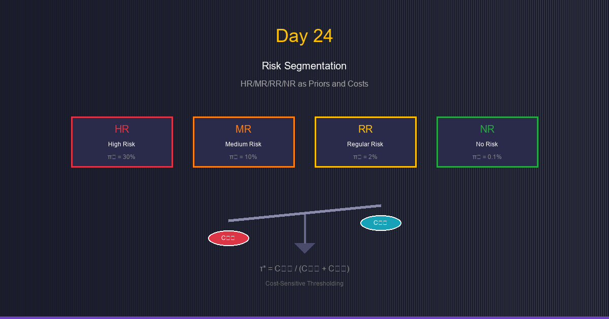
Interpret priority tiers as prior beliefs or cost weights. Learn cost-sensitive thresholding and Bayes optimal decisions.
When different types of errors have different costs, a single threshold isn't optimal. Risk segmentation lets us tune decisions per segment, balancing precision and recall based on business needs.
The Problem: One Threshold Doesn't Fit All
Scenario: You have an anomaly detection system with four priority tiers:
- Critical: High-priority entities requiring immediate attention
- High: Elevated concern, needs investigation
- Standard: Normal entities, low anomaly rate
- Baseline: Verified trusted entities, minimal intervention
Question: Should you use the same decision threshold for all tiers?
Answer: No! Different tiers have different:
- Prior probabilities (base rates of anomalies)
- Misclassification costs (cost of false positives vs false negatives)
The insight: Priority tiers encode our prior beliefs and cost preferences!
Priority Tiers as Prior Beliefs
What are Priors?
Prior probability (π) is our belief about class proportions before seeing the score.
Notation:
- π₁ = P(Anomaly) = Prior probability of positive class
- π₀ = P(Normal) = Prior probability of negative class
- π₀ + π₁ = 1
Different Priors by Priority Tier
Example:
Tier       π₁ (Anomaly Rate)    π₀ (Normal)

Critical   0.30 (30%)           0.70 (70%)
High       0.10 (10%)           0.90 (90%)
Standard   0.02 (2%)            0.98 (98%)
Baseline   0.001 (0.1%)         0.999 (99.9%)
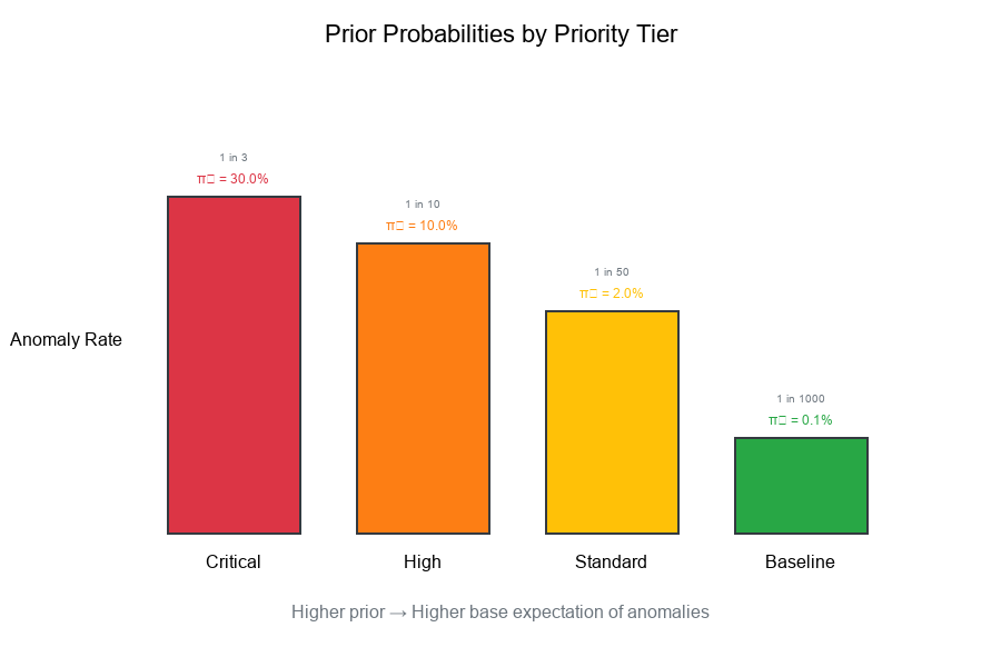
Interpretation:
- Critical: 1 in 3 events is an anomaly (high prior)
- High: 1 in 10 events is an anomaly
- Standard: 1 in 50 events is an anomaly
- Baseline: 1 in 1000 events is an anomaly (very low prior)
Visual Example:
Priority Tiers as Cost Weights
Misclassification Costs
Not all errors are equal! We define:
- C₀₁ (False Positive Cost): Cost of flagging a normal entity
- Wasted resources, unnecessary investigation, user friction
- C₁₀ (False Negative Cost): Cost of missing an anomaly
- Missed opportunity, undetected issue, downstream impact
Cost Matrix
Predicted
Negative  Positive
Actual  Negative    0        C₀₁
Positive   C₁₀        0
Different Costs by Priority Tier
Example:
Tier       C₁₀ (Miss Anomaly)    C₀₁ (False Alarm)    Ratio C₁₀/C₀₁

Critical   $10,000               $50                  200:1
High       $5,000                $100                 50:1
Standard   $1,000                $200                 5:1
Baseline   $500                  $500                 1:1
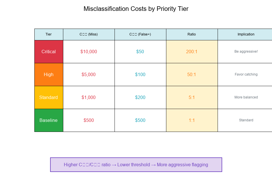
Interpretation:
- Critical: Missing anomaly is 200× worse than false alarm → Be aggressive!
- High: Missing anomaly is 50× worse → Still favor catching anomalies
- Standard: Missing anomaly is 5× worse → More balanced
- Baseline: Costs are equal → Standard threshold
Visual Example:
Cost-Sensitive Thresholding
The Standard Threshold
Without cost considerations, we typically use τ = 0.5:
- If P(Anomaly|x) ≥ 0.5, predict Positive
- If P(Anomaly|x) < 0.5, predict Negative
The Bayes Optimal Threshold
With unequal costs and priors, the optimal threshold shifts!
Bayes Decision Rule:
Predict Positive (Anomaly) if:
P(Anomaly|x) · C₁₀ > P(Normal|x) · C₀₁
Rearranging:
P(Anomaly|x) / P(Normal|x) > C₀₁ / C₁₀
Using odds notation:
Odds(Anomaly|x) > C₀₁ / C₁₀
Deriving the Threshold
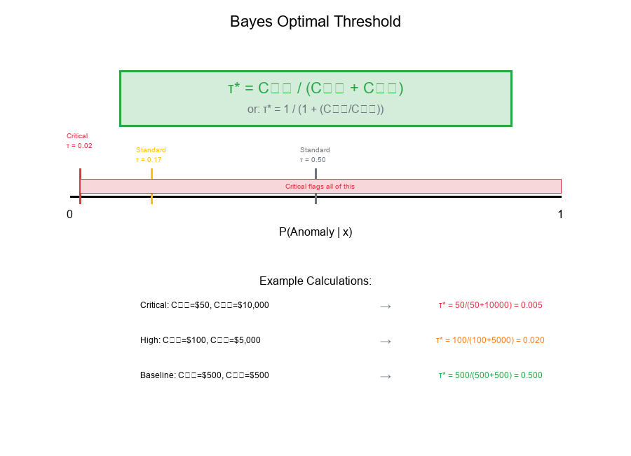
Optimal Threshold Formula:
τ* = C₀₁ / (C₀₁ + C₁₀)
Or equivalently, incorporating priors:
τ* = 1 / (1 + (C₁₀/C₀₁) · (π₁/π₀))
Alternative form (likelihood ratio threshold):
τ_LR = (C₀₁/C₁₀) · (π₀/π₁)
Visual Example:
Per-Tier Thresholds: Changing Labeling Geometry
Computing Tier-Specific Thresholds
Using the formula τ* = C₀₁ / (C₀₁ + C₁₀):
Tier       C₁₀      C₀₁     τ* = C₀₁/(C₀₁+C₁₀)

Critical   $10,000  $50     50/(50+10000) = 0.005
High       $5,000   $100    100/(100+5000) = 0.020
Standard   $1,000   $200    200/(200+1000) = 0.167
Baseline   $500     $500    500/(500+500) = 0.500
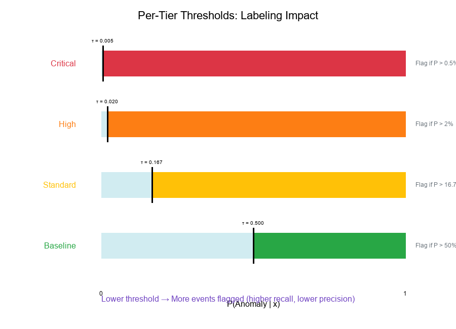
Interpretation:
- Critical (τ = 0.005):* Flag anything with >0.5% anomaly probability
- High (τ = 0.020):* Flag anything with >2% anomaly probability
- Standard (τ = 0.167):* Flag anything with >16.7% anomaly probability
- Baseline (τ = 0.500):* Standard 50% threshold
Impact on Labeling
Lower threshold → More events flagged (higher recall, lower precision) Higher threshold → Fewer events flagged (higher precision, lower recall)
Visual Example:
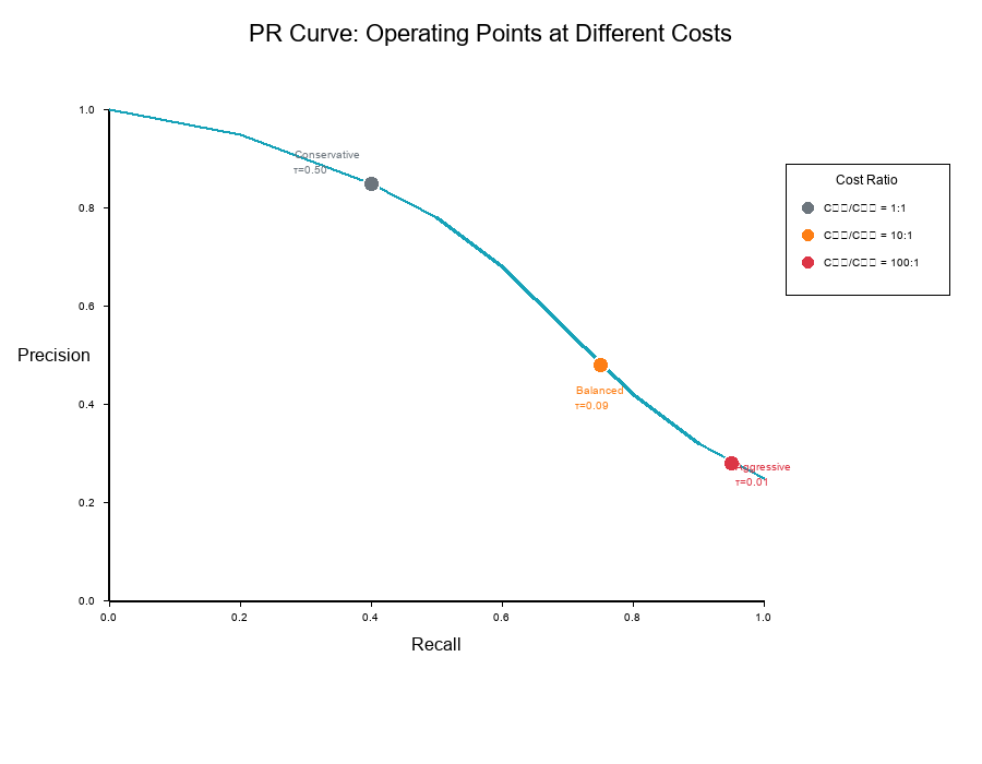
Visualizing: PR Curves at Different Costs
What Changes with Cost?
The same model produces different operating points when costs change.
On a Precision-Recall curve:
- Each threshold corresponds to a (Precision, Recall) point
- Different costs select different optimal points
- Higher C₁₀/C₀₁ ratio → Move toward higher recall
Three Operating Points
Example with three cost scenarios:
Scenario         C₁₀/C₀₁    Optimal τ    Precision    Recall

Conservative     1:1        0.50         85%          40%
Balanced         10:1       0.09         60%          75%
Aggressive       100:1      0.01         30%          95%
Visual Example:
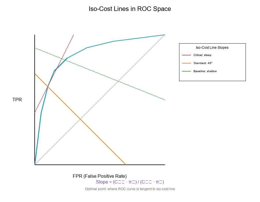
Iso-Cost Lines: Visualizing Cost Trade-offs
What are Iso-Cost Lines?
Iso-cost lines connect points with equal expected cost on the ROC or PR space.
Formula (ROC space):
Expected Cost = C₀₁ · π₀ · FPR + C₁₀ · π₁ · FNR
= C₀₁ · π₀ · FPR + C₁₀ · π₁ · (1 - TPR)
For constant cost C:
TPR = 1 - (C - C₀₁ · π₀ · FPR) / (C₁₀ · π₁)
This is a linear equation with slope:
slope = (C₀₁ · π₀) / (C₁₀ · π₁)
Reading Iso-Cost Lines
Properties:
- Lines closer to top-left corner = lower cost
- Slope depends on cost ratio and priors
- Optimal point = where ROC curve is tangent to iso-cost line
Different slopes for different tiers:
Tier       Slope = (C₀₁·π₀)/(C₁₀·π₁)

Critical   (50·0.70)/(10000·0.30) = 0.012
High       (100·0.90)/(5000·0.10) = 0.18
Standard   (200·0.98)/(1000·0.02) = 9.8
Baseline   (500·0.999)/(500·0.001) = 999
Visual Example:
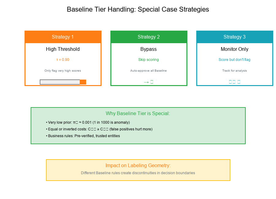
Baseline Tier Handling: Special Case
What Makes Baseline Different?
Baseline tier entities often receive special treatment:
- Very low prior: π₁ ≈ 0.001 or less
- Equal or inverted costs: C₀₁ ≥ C₁₀ (false positives hurt more)
- Business rules: May bypass scoring entirely
Baseline Handling Strategies
Strategy 1: High Threshold
τ_baseline = 0.90 (Only flag very high scores)
Strategy 2: Bypass
if tier == "Baseline":
return "Auto-Approve"  # Skip scoring
Strategy 3: Score but Don't Flag
# Score for monitoring, but don't take action
if tier == "Baseline":
tag = "Monitor-Only"
Impact on Labeling Geometry
When Baseline uses different rules:
- The decision boundary shifts dramatically
- Creates discontinuity in the overall labeling
- Requires careful tracking of tier-specific metrics
Visual Example:
Real-World Application: Per-Tier Threshold Configuration
Configuration Structure
Show code (31 lines)
tier_config = {
'Critical': {
'prior': 0.30,
'cost_fn': 10000,  # C₁₀: cost of missing anomaly
'cost_fp': 50,     # C₀₁: cost of false positive
'threshold': 0.005,
'action': 'flag_for_review'
},
'High': {
'prior': 0.10,
'cost_fn': 5000,
'cost_fp': 100,
'threshold': 0.020,
'action': 'flag_for_review'
},
'Standard': {
'prior': 0.02,
'cost_fn': 1000,
'cost_fp': 200,
'threshold': 0.167,
'action': 'flag_if_above'
},
'Baseline': {
'prior': 0.001,
'cost_fn': 500,
'cost_fp': 500,
'threshold': 0.500,
'action': 'auto_approve'
}
}
Applying Per-Tier Thresholds
Show code (23 lines)
def apply_tier_threshold(event, score, tier_config):
"""
Apply tier-specific threshold to determine action.

Parameters:
- event: Event dictionary with 'priority_tier'
- score: Model score (probability)
- tier_config: Configuration dictionary

Returns:
- action: 'flag', 'approve', or 'monitor'
"""
tier = event['priority_tier']
config = tier_config[tier]
threshold = config['threshold']

if config['action'] == 'auto_approve':
return 'approve'
elif score >= threshold:
return 'flag'
else:
return 'approve'
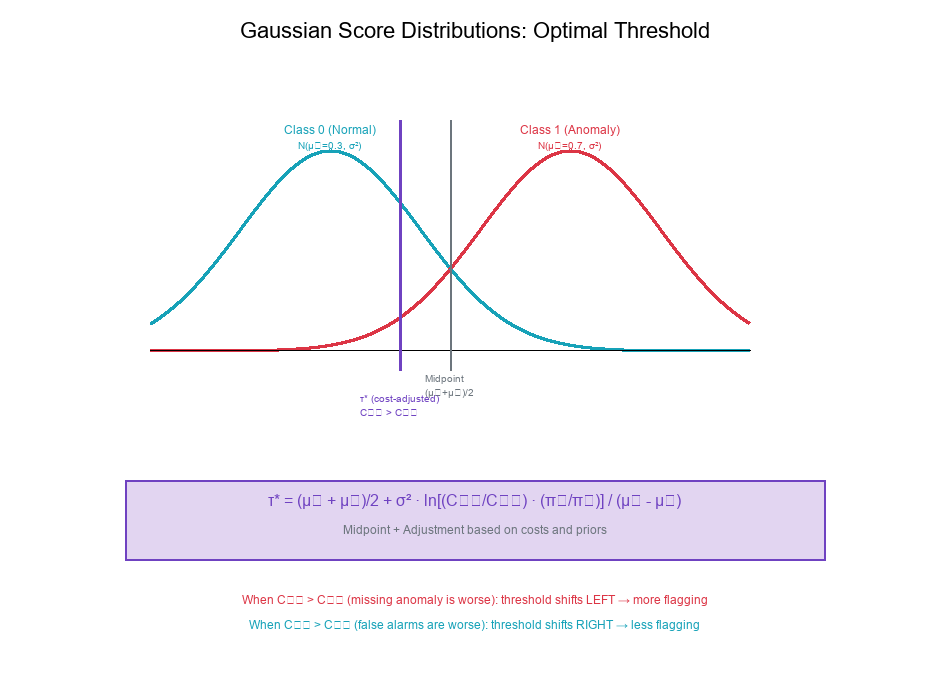
Exercise: Deriving the Decision Threshold
The Problem
Given:
- Two classes with Gaussian score distributions
- Class 0 (Normal): N(μ₀, σ²)
- Class 1 (Anomaly): N(μ₁, σ²) where μ₁ > μ₀
- Priors: π₀, π₁
- Costs: C₀₁ (false positive), C₁₀ (false negative)
Derive: The optimal decision threshold τ*
Solution
Step 1: Bayes Decision Rule
Predict Class 1 (Anomaly) if:
π₁ · P(x|Class 1) · C₁₀ > π₀ · P(x|Class 0) · C₀₁
Step 2: Likelihood Ratio
Rearranging:
P(x|Class 1) / P(x|Class 0) > (C₀₁/C₁₀) · (π₀/π₁)
Let λ = (C₀₁/C₁₀) · (π₀/π₁) be the threshold likelihood ratio.
Step 3: Gaussian Likelihood Ratio
For Gaussian distributions with equal variance:
P(x|Class 1) / P(x|Class 0) = exp[-(x-μ₁)²/2σ² + (x-μ₀)²/2σ²]
= exp[(μ₁-μ₀)(2x-μ₁-μ₀) / 2σ²]
Step 4: Solve for Threshold
Setting likelihood ratio = λ:
(μ₁-μ₀)(2x-μ₁-μ₀) / 2σ² = ln(λ)
Solving for x:
τ* = (μ₁ + μ₀)/2 + σ² · ln(λ) / (μ₁ - μ₀)
Step 5: Simplify
Substituting λ = (C₀₁/C₁₀) · (π₀/π₁):
τ* = (μ₁ + μ₀)/2 + σ² · ln[(C₀₁/C₁₀) · (π₀/π₁)] / (μ₁ - μ₀)
Interpretation
The optimal threshold has two components:
- Midpoint: (μ₁ + μ₀)/2 — where distributions cross
- Shift: Adjustment based on costs and priors
When C₁₀ > C₀₁ (missing anomaly is worse):
- λ < 1, ln(λ) < 0
- Threshold shifts left (lower)
- More events flagged
When π₁ > π₀ (anomalies are common):
- λ smaller
- Threshold shifts left
- More events flagged
Visual Example:
Best Practices for Tier-Based Thresholding
1. Estimate Priors Carefully
- Use historical data to estimate tier-specific anomaly rates
- Update priors regularly as patterns change
- Consider seasonal variations
2. Quantify Costs Explicitly
- Work with business stakeholders to define costs
- Include both direct and indirect costs
- Document assumptions
3. Validate Thresholds Empirically
- Backtest on historical data
- Monitor performance by tier
- Adjust based on observed outcomes
4. Handle Edge Cases
- Define behavior for missing tiers
- Plan for new/unknown priority categories
- Set sensible defaults
5. Document Everything
- Record threshold derivations
- Track cost assumptions
- Log threshold changes over time
6. Monitor Tier Drift
- Watch for changes in tier composition
- Alert on significant prior shifts
- Recalibrate periodically
Summary Table
| Concept | Formula | Description |
|---|---|---|
| Prior Probability | π₁ = P(Anomaly) | Base rate of positive class |
| Cost Ratio | C₁₀ / C₀₁ | How much worse is missing anomaly vs false alarm |
| Bayes Threshold | τ* = C₀₁ / (C₀₁ + C₁₀) | Cost-optimal decision boundary |
| Likelihood Ratio | λ = (C₀₁/C₁₀) · (π₀/π₁) | Threshold in likelihood space |
| Iso-Cost Slope | (C₀₁ · π₀) / (C₁₀ · π₁) | Slope of equal-cost lines in ROC |
| Gaussian Threshold | (μ₁+μ₀)/2 + adjustment | Optimal threshold for Gaussian scores |
Final Thoughts
Risk segmentation transforms a one-size-fits-all approach into a nuanced, cost-aware decision system. By treating priority tiers as carriers of prior beliefs and cost weights, we can:
- Optimize decisions per tier
- Balance trade-offs explicitly
- Allocate resources efficiently
- Communicate rationale clearly
Key Takeaways:
Priority tiers encode priors — different base rates for different tiers Costs drive thresholds — higher stakes → more aggressive flagging Bayes optimal threshold — τ* = C₀₁ / (C₀₁ + C₁₀) Iso-cost lines — visualize cost trade-offs in ROC/PR space Baseline handling — special rules for trusted tiers Gaussian derivation — τ* = midpoint + cost/prior adjustment
Match your thresholds to your costs!