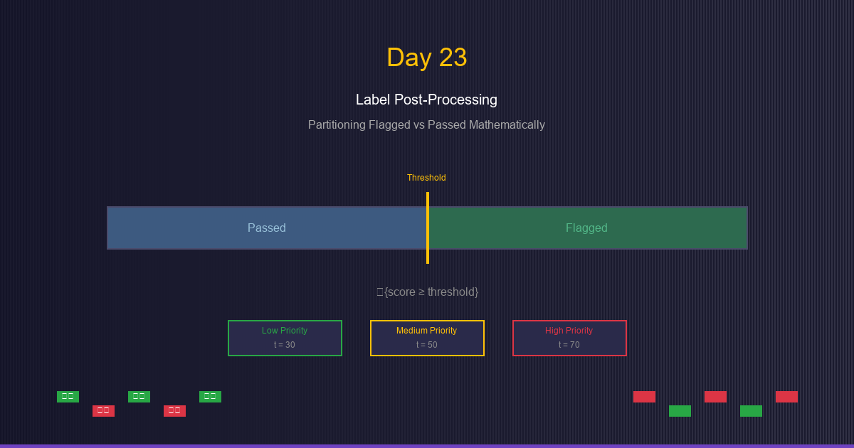
Day 23: Label Post-Processing: Partitioning Flagged vs Passed Mathematically
See event tagging as rule-based classification. Learn to mathematically partition events using indicator functions and piecewise rules.
When working with scores and event classifications, we often need to partition data into distinct categories. Understanding the mathematical foundations of these partitions helps us reason about rule behavior and ensure consistency.
The Problem: Event Tagging as Classification
Scenario: You have a scoring system that produces continuous scores (0-100). You need to decide:
- Which events get Flagged → Require human review
- Which events get Passed → Auto-approved or processed
Challenge: How do you mathematically define and reason about these partitions?
Example:
Raw scores: [23, 67, 45, 89, 12, 55, 78, 34]
Threshold: 50

Flagged (score ≥ 50): [67, 89, 55, 78] → 4 events (50%)
Passed (score < 50):  [23, 45, 12, 34] → 4 events (50%)
The question: How do we formalize this mathematically?
Indicator Functions: The Building Blocks
What is an Indicator Function?
An indicator function (also called a characteristic function) is a function that returns 1 if a condition is true, and 0 otherwise.
Notation:
{condition} = {
1, if condition is true
0, if condition is false
}
Also written as:
I(condition)1_A(indicator of set A)[condition](Iverson bracket)
Examples of Indicator Functions
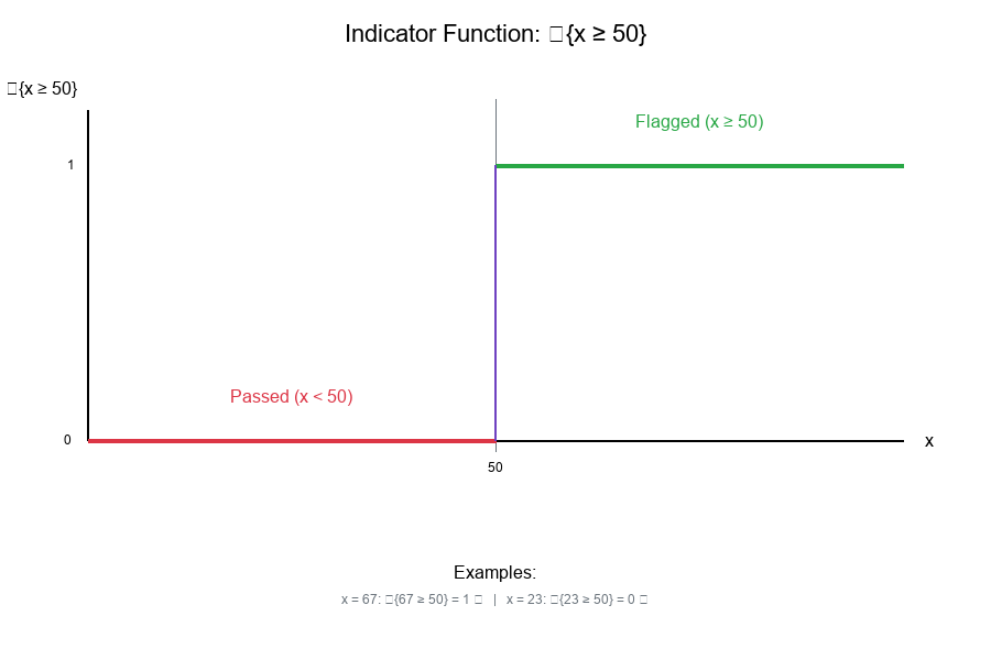
Example 1: Simple Threshold
{x ≥ 50} = {
1, if x ≥ 50
0, if x < 50
}

For x = 67: {67 ≥ 50} = 1
For x = 23: {23 ≥ 50} = 0
Example 2: Range Check
{30 ≤ x < 70} = {
1, if 30 ≤ x < 70
0, otherwise
}

For x = 45: {30 ≤ 45 < 70} = 1
For x = 80: {30 ≤ 80 < 70} = 0
Visual Example:
Indicator Functions for Inequalities
Common Inequality Patterns
Greater Than or Equal:
{x ≥ t} = {
1, if x ≥ t
0, if x < t
}
Less Than:
{x < t} = {
1, if x < t
0, if x ≥ t
}
Complement Property:
{x < t} = 1 - {x ≥ t}
Double-Sided (Range):
{a ≤ x < b} = {x ≥ a} · {x < b}
Flagged vs Passed with Indicator Functions
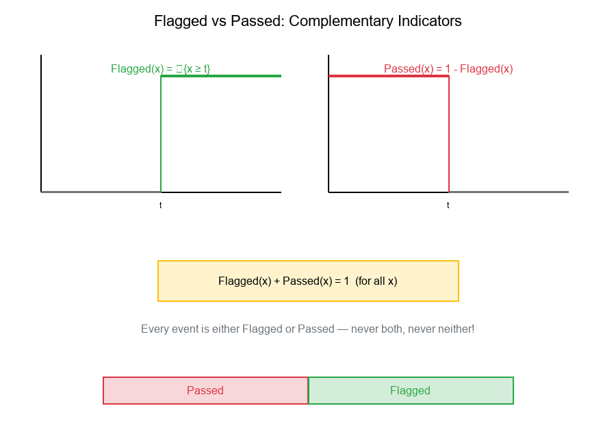
Definition:
Flagged(x) = {x ≥ threshold}
Passed(x) = {x < threshold} = 1 - Flagged(x)
Key Property: Partition
Flagged(x) + Passed(x) = 1 (for all x)
This means every event is either Flagged or Passed—never both, never neither!
Visual Example:
Piecewise Partitions: Multiple Categories
What is a Piecewise Partition?
A piecewise partition divides the domain into multiple non-overlapping regions, each handled by a different rule.
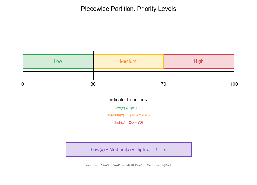
Example: Priority Levels
Priority Level(x) = {
"Low",      if x < 30
"Medium",   if 30 ≤ x < 70
"High",     if x ≥ 70
}
Mathematical Representation
Using indicator functions:
Low(x)    = {x < 30}
Medium(x) = {30 ≤ x < 70}
High(x)   = {x ≥ 70}
Partition Property:
Low(x) + Medium(x) + High(x) = 1 (for all x)
General Form
For thresholds t₁ < t₂ < ... < tₙ:
Region₀(x) = {x < t₁}
Region₁(x) = {t₁ ≤ x < t₂}
Region₂(x) = {t₂ ≤ x < t₃}
...
Regionₙ(x) = {x ≥ tₙ}
Visual Example:
Priority-Level Conditioning
What is Priority-Level Conditioning?
Priority-level conditioning means applying different rules based on the priority level of an event.
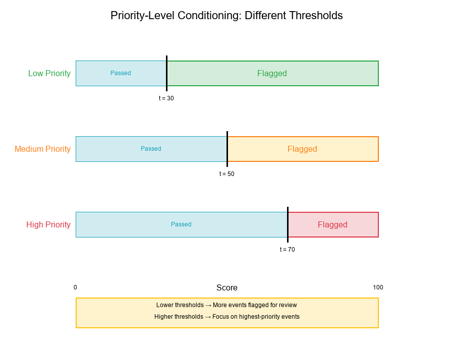
Example:
Flag_rule(x, priority) = {
{x ≥ 30},  if priority = "Low"     (lower threshold for low priority)
{x ≥ 50},  if priority = "Medium"  (standard threshold)
{x ≥ 70},  if priority = "High"    (higher threshold for high priority)
}
Mathematical Formulation
Let P(x) be the priority level function. The conditioned Flag rule is:
Flagged(x) = {P(x) = "Low"} · {x ≥ 30}
+ {P(x) = "Medium"} · {x ≥ 50}
+ {P(x) = "High"} · {x ≥ 70}
Interpretation:
- Low-priority events: Flagged if score ≥ 30
- Medium-priority events: Flagged if score ≥ 50
- High-priority events: Flagged if score ≥ 70
Why Different Thresholds?
Rationale:
- Low-priority segments: More conservative, flag more events
- High-priority segments: More aggressive, focus on highest scores
- Resource allocation: Direct review resources where they matter most
Visual Example:
Real-World Application: partition_events_by_thresholds
Purpose
The partition_events_by_thresholds function applies tuned rules and updates tags for each event.
Use Cases:
- Classify events into Flagged/Passed categories
- Apply priority-level specific thresholds
- Update event labels based on post-processing rules
- Track before/after tag distributions
Function Concept
Show code (26 lines)
def partition_events_by_thresholds(events, thresholds, priority_levels):
"""
Partition events into Flagged/Passed based on thresholds and priority levels.

Parameters:
- events: List of event dictionaries with 'score' and 'priority_level'
- thresholds: Dict mapping priority levels to thresholds
- priority_levels: List of priority levels to consider

Returns:
- events: Updated with 'tag' field (Flagged or Passed)
- stats: Before/after class proportions per priority level
"""
for event in events:
priority = event['priority_level']
score = event['score']
threshold = thresholds.get(priority, 50)  # Default threshold

# Apply indicator function
if score >= threshold:
event['tag'] = 'Flagged'
else:
event['tag'] = 'Passed'

return events, compute_stats(events, priority_levels)
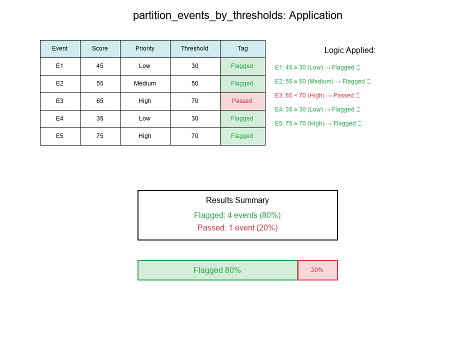
Example Application
Input:
Show code (14 lines)
events = [
{'id': 1, 'score': 45, 'priority_level': 'Low'},
{'id': 2, 'score': 55, 'priority_level': 'Medium'},
{'id': 3, 'score': 65, 'priority_level': 'High'},
{'id': 4, 'score': 35, 'priority_level': 'Low'},
{'id': 5, 'score': 75, 'priority_level': 'High'},
]

thresholds = {
'Low': 30,
'Medium': 50,
'High': 70
}
Output:
Show code (10 lines)
# Event 1: score=45, priority=Low, threshold=30 → 45 ≥ 30 → Flagged
# Event 2: score=55, priority=Medium, threshold=50 → 55 ≥ 50 → Flagged
# Event 3: score=65, priority=High, threshold=70 → 65 < 70 → Passed
# Event 4: score=35, priority=Low, threshold=30 → 35 ≥ 30 → Flagged
# Event 5: score=75, priority=High, threshold=70 → 75 ≥ 70 → Flagged

# Results:
# Flagged: [Event 1, Event 2, Event 4, Event 5] → 4 events (80%)
# Passed: [Event 3] → 1 event (20%)
Visual Example:
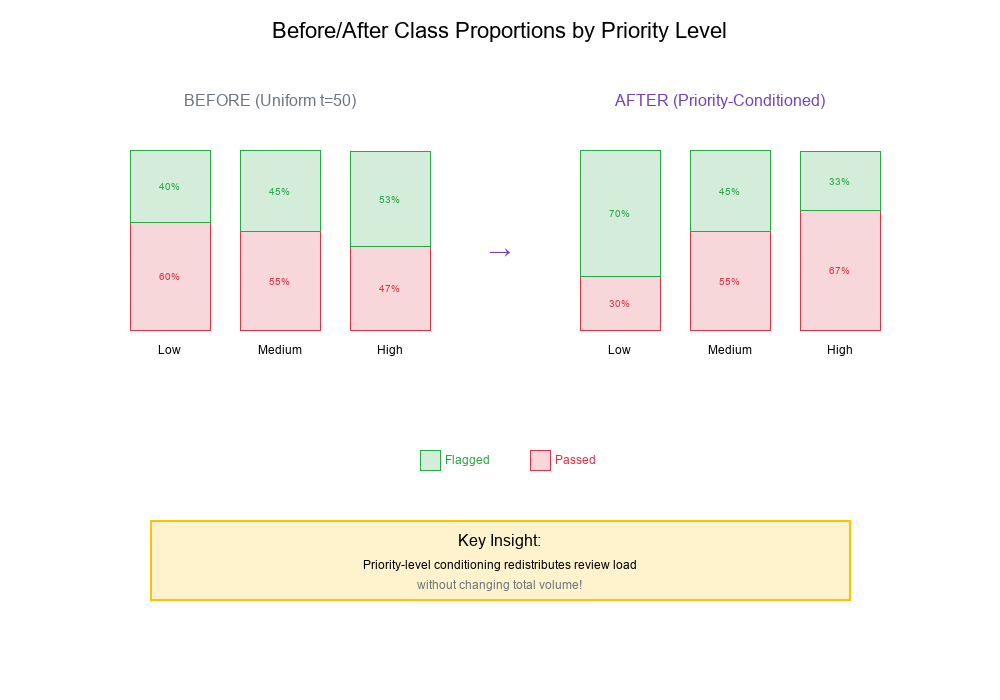
Before/After Class Proportions
Visualizing the Impact
When you apply post-processing rules, it's crucial to visualize the before/after class proportions.
Example Scenario:
Before (Uniform Threshold = 50):
Priority Level  Total  Flagged  Passed  Flagged%

Low             1000     400     600      40%
Medium          2000     900    1100      45%
High            1500     800     700      53%

Total           4500    2100    2400      47%
After (Priority-Conditioned Thresholds):
Show code (10 lines)
Thresholds: Low=30, Medium=50, High=70

Priority Level  Total  Flagged  Passed  Flagged%

Low             1000     700     300      70%  ↑ More review
Medium          2000     900    1100      45%  = Same
High            1500     500    1000      33%  ↓ Less review

Total           4500    2100    2400      47%  = Same total!
Key Insight: Priority-level conditioning redistributes review load without changing total volume!
Visual Example:
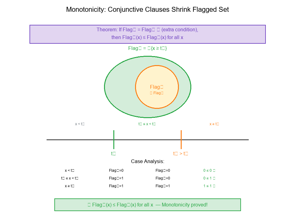
Exercise: Monotonicity of Conjunctive Clauses
The Problem
Theorem: Adding a conjunctive clause can only shrink the Flagged set.
Claim: If we define:
Flag₁(x) = {x ≥ t₁}
Flag₂(x) = {x ≥ t₁} · {x ≥ t₂}  (where t₂ > t₁)
Then: Flag₂(x) ≤ Flag₁(x) for all x.
Prove this monotonicity property.
Solution
Step 1: Analyze Flag₁
Flag₁(x) = {x ≥ t₁} = {
1, if x ≥ t₁
0, if x < t₁
}
Step 2: Analyze Flag₂
Flag₂(x) = {x ≥ t₁} · {x ≥ t₂}
Since t₂ > t₁, the condition x ≥ t₂ implies x ≥ t₁.
Therefore:
Flag₂(x) = {
1, if x ≥ t₂ (which implies x ≥ t₁)
0, otherwise
}
Step 3: Compare
Case analysis for all x:
| Case | x < t₁ | t₁ ≤ x < t₂ | x ≥ t₂ | |------|--------|-------------|--------| | Flag₁ | 0 | 1 | 1 | | Flag₂ | 0 | 0 | 1 | | Flag₂ ≤ Flag₁? | (0 ≤ 0) | (0 ≤ 1) | (1 ≤ 1) |
Step 4: Conclusion
For all x: Flag₂(x) ≤ Flag₁(x)
Interpretation: Adding the extra condition x ≥ t₂ (where t₂ > t₁) can only make it harder to be Flagged, never easier. This is the monotonicity property of conjunctive clauses.
General Principle
Monotonicity of AND:
If C = A ∧ B, then:
- C can only be true when BOTH A and B are true
- C ⊆ A and C ⊆ B
- |C| ≤ min(|A|, |B|)
Practical Implication:
- Adding more conditions to a rule can only reduce the set of matching events
- Never increase it
- This is useful for understanding rule refinement
Visual Example:
Practical Applications
1. Rule Refinement
Scenario: Current Flagged rule catches too many false positives.
Solution: Add conjunctive clauses to narrow down:
Before: Flagged = {score ≥ 50}
After:  Flagged = {score ≥ 50} · {amount ≥ 1000}
Guaranteed: New Flagged ⊆ Old Flagged (monotonicity)
2. A/B Testing Rules
Scenario: Testing a new threshold.
Approach:
- Define Flag_control and Flag_treatment
- Use indicator functions to track differences
- Measure
|Flag_control ⊕ Flag_treatment|(symmetric difference)
3. Threshold Calibration
Scenario: Adjusting thresholds per priority level.
Method:
- Start with uniform threshold
- Apply priority-level conditioning
- Monitor before/after proportions
- Iterate until balanced
Best Practices for Label Post-Processing
1. Document Your Rules Mathematically
Write rules as indicator functions to:
- Ensure clarity
- Enable formal reasoning
- Detect logical errors
2. Verify Partition Properties
Always check that:
∑ Category_i(x) = 1 for all x
Every event belongs to exactly one category.
3. Track Before/After Proportions
Monitor class distributions:
- Per priority level
- Per segment
- Over time
4. Understand Monotonicity
When adding conditions:
- Conjunctive (AND): Shrinks the set
- Disjunctive (OR): Expands the set
5. Test Edge Cases
Check behavior at:
- Exact threshold values
- Boundary conditions
- Missing data scenarios
6. Version Control Your Rules
Track rule changes:
- What changed
- When it changed
- Why it changed
- Impact on proportions
Summary Table
| Concept | Notation | Description | Use Case |
|---|---|---|---|
| Indicator Function | {condition} |
Returns 1 if true, 0 if false | Binary classification |
| Flagged Indicator | {x ≥ t} |
Above threshold check | Review flagging |
| Passed Indicator | 1 - {x ≥ t} |
Below threshold (complement) | Auto-processing |
| Piecewise Partition | ∑ Region_i = 1 | Non-overlapping regions | Multi-category classification |
| Priority Conditioning | Flagged(x, priority) | Different thresholds per priority | Segment-specific rules |
| Monotonicity | A ∧ B ⊆ A | AND shrinks sets | Rule refinement |
Final Thoughts
Label post-processing is fundamentally about applying mathematical rules to partition events into categories. By formalizing these rules with indicator functions, we gain:
- Clarity: Precise definitions that eliminate ambiguity
- Reasoning: Ability to prove properties like monotonicity
- Consistency: Guaranteed partitions where every event has exactly one category
- Insight: Before/after comparisons that reveal rule impact
Key Takeaways:
Indicator functions are the building blocks of rule-based classification Piecewise partitions divide the score space into non-overlapping regions Priority-level conditioning allows segment-specific thresholds partition_events_by_thresholds applies tuned rules and updates tags Before/after proportions reveal the impact of rule changes Conjunctive clauses can only shrink the Flagged set (monotonicity)
Think mathematically about your rules!
Where This Shows Up in Practice
- Data Pipelines: Ensuring high-quality filtering and robust statistical metrics before feeding downstream ML models.
- Production Anomaly Detection: Tracking system logs, performance latencies, or transaction volumes under heavy skew.
- A/B Testing & Evaluation: Correctly partitioning user cohorts or comparing treatment outcomes without normal distribution assumptions.