Day 27: Quantile Stability, Ties, and Small Samples
The Problem: Quantiles in Practice
Scenario: You're computing the 90th percentile threshold from transaction data.
Challenges:
- Ties: Multiple transactions have the same value
- Discrete data: Values are integers (counts) or categorical
- Small samples: Only 50 observations available
- Interpolation: Different methods give different answers!
Question: How do you get stable, repeatable quantile estimates?
The Empirical CDF (ECDF)
Definition
The empirical cumulative distribution function gives the proportion of observations ≤ x:
F̂_n(x) = (1/n) × |{i : X_i ≤ x}|
Properties:
- Step function (jumps at data points)
- F̂_n(x) ∈ [0, 1]
- F̂_n(-∞) = 0, F̂_n(∞) = 1
ECDF with Ties
With ties: Multiple observations at the same value create larger jumps.
Example:
Show code (9 lines)
Data: [1, 2, 2, 2, 3, 4, 5]  (n = 7)

ECDF:
F̂(1) = 1/7 = 0.143
F̂(2) = 4/7 = 0.571  (3 values = 2, plus 1 below)
F̂(3) = 5/7 = 0.714
F̂(4) = 6/7 = 0.857
F̂(5) = 7/7 = 1.000
Visual Example:
Quantile Definition: Multiple Methods
The Quantile Inverse Problem
Goal: Find x such that F̂_n(x) = p
Problem: ECDF is a step function—F̂_n(x) = p may have:
- No solution (p falls in a gap)
- Infinite solutions (p falls on a flat step)
Interpolation Schemes
There are at least 9 different quantile definitions!
Common methods:
Type 1: Inverse of ECDF (closest observation)
Q(p) = X_(⌈np⌉)
Type 6: Linear interpolation (Excel)
Q(p) = X_(j) + (X_(j+1) - X_(j)) × (np + 0.5 - j)
where j = ⌊np + 0.5⌋
Type 7: Linear interpolation (R/Python default)
Q(p) = X_(j) + (X_(j+1) - X_(j)) × (np + 1 - p - j)
where j = ⌊(n-1)p + 1⌋
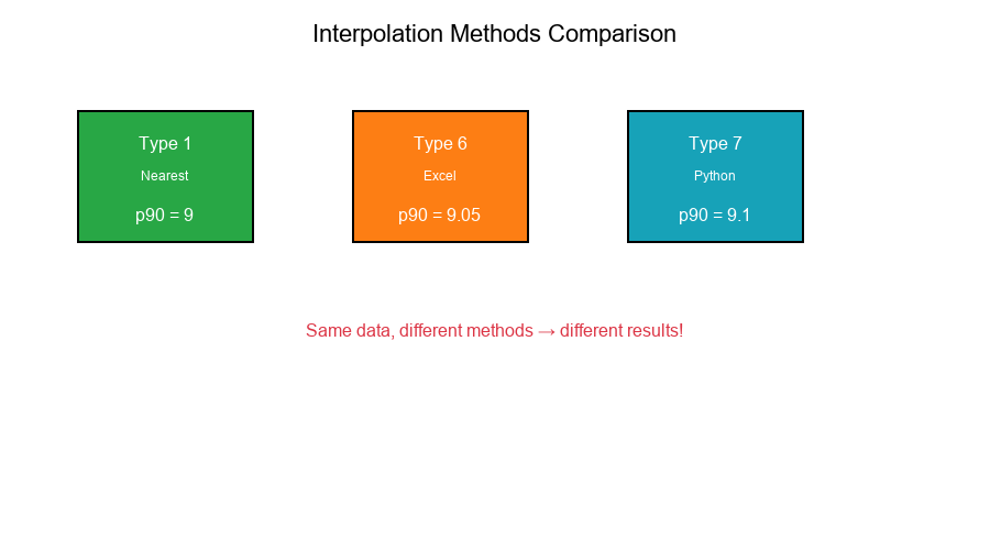
Why It Matters
Example: n = 10, find 90th percentile
Data: [1, 2, 3, 4, 5, 6, 7, 8, 9, 10]
| Method | Formula | Result |
|---|---|---|
| Type 1 | X_(⌈9⌉) = X_9 | 9 |
| Type 6 | Interpolate | 9.05 |
| Type 7 | Interpolate | 9.1 |
Visual Example:
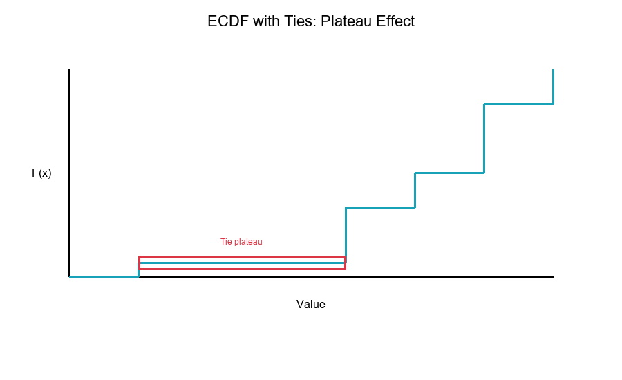
Ties: The Plateau Problem
What Happens with Ties?
When multiple observations have the same value, the ECDF has a flat plateau.
Problem: The quantile is non-unique at the plateau level.
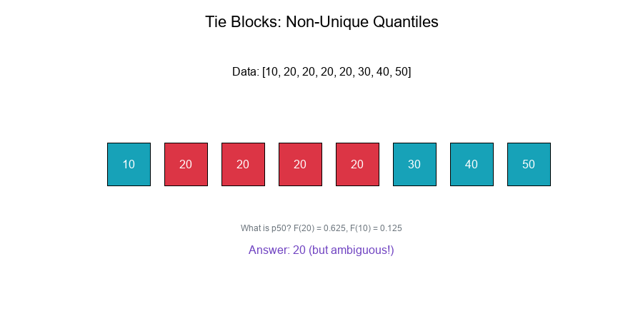
Example with Ties
Data: [10, 20, 20, 20, 20, 30, 40, 50] (n = 8)
ECDF:
F̂(10) = 1/8 = 0.125
F̂(20) = 5/8 = 0.625  ← Plateau from 0.125 to 0.625
F̂(30) = 6/8 = 0.750
F̂(40) = 7/8 = 0.875
F̂(50) = 8/8 = 1.000
What is the 50th percentile?
- F̂(20) = 0.625 > 0.50
- F̂(10) = 0.125 < 0.50
- Answer: 20 (but could argue for values between 10 and 20)
Handling Ties
Strategies:
- Left-continuous: Q(p) = inf{x : F̂(x) ≥ p}
- Right-continuous: Q(p) = inf{x : F̂(x) > p}
- Midpoint: Average of left and right
- Random jitter: Add small noise to break ties
Visual Example:
Small Sample Variance
Quantile Variance
Quantile estimates have variance that depends on:
- Sample size n
- The quantile level p
- The density at the quantile f(Q_p)
Asymptotic variance:
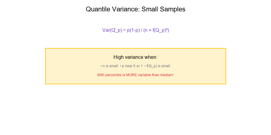
Var(Q̂_p) ≈ p(1-p) / (n × f(Q_p)²)
Implications
High variance when:
- n is small
- p is extreme (near 0 or 1)
- f(Q_p) is small (sparse region)
Example:
n = 50, p = 0.90

Variance factor = 0.90 × 0.10 / 50 = 0.0018

For p = 0.50:
Variance factor = 0.50 × 0.50 / 50 = 0.0050
The 90th percentile is more variable than the median!
Confidence Intervals
Bootstrap confidence interval for quantiles:
Show code (13 lines)
def quantile_bootstrap_ci(data, p, n_bootstrap=1000, alpha=0.05):
n = len(data)
quantiles = []

for _ in range(n_bootstrap):
sample = np.random.choice(data, size=n, replace=True)
quantiles.append(np.percentile(sample, p * 100))

lower = np.percentile(quantiles, alpha/2 * 100)
upper = np.percentile(quantiles, (1 - alpha/2) * 100)

return lower, upper
Visual Example:
Closest Observation Method
What is It?
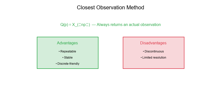
The closest observation method (Type 1) returns the actual data value closest to the theoretical quantile.
Formula:
Q(p) = X_(⌈np⌉)
Advantages
- Repeatability: Always returns an actual observation
- Stability: Less sensitive to interpolation choices
- Discrete-friendly: Works well with integer data
Disadvantages
- Discontinuous: Jumps as p varies
- Limited resolution: Restricted to n possible values
- Bias: May systematically over/underestimate
Implementation
Show code (10 lines)
def quantile_closest(data, p):
"""
Closest observation quantile (Type 1).
"""
sorted_data = np.sort(data)
n = len(data)
index = int(np.ceil(n * p)) - 1  # 0-based index
index = max(0, min(index, n - 1))  # Clamp to valid range
return sorted_data[index]
Visual Example:
Repeatability of Thresholds
Why Repeatability Matters
Scenario: You compute a threshold today and again tomorrow.
Question: Will you get the same value?
Factors affecting repeatability:
- Data changes: New observations added
- Tie handling: Ambiguous quantile definition
- Interpolation method: Different software defaults
- Floating-point precision: Numerical issues
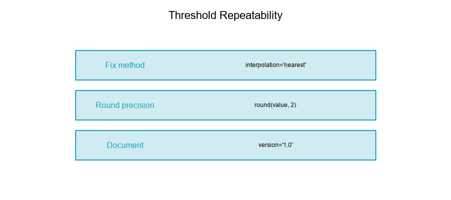
Strategies for Repeatability
1. Fix the interpolation method:
# Always use the same method
threshold = np.percentile(data, 90, interpolation='nearest')
2. Use closest observation:
# Returns actual data value
threshold = np.percentile(data, 90, interpolation='lower')
3. Round to meaningful precision:
# Avoid floating-point issues
threshold = round(np.percentile(data, 90), 2)
4. Document the method:
QUANTILE_CONFIG = {
'method': 'nearest',
'precision': 2,
'version': '1.0'
}
Visual Example:
Exercise: Comparing Interpolation Rules
The Problem
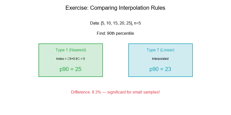
Given: A tiny sample: [5, 10, 15, 20, 25] (n = 5)
Compute: The 90th percentile under two interpolation rules:
- Type 1 (nearest/ceiling)
- Type 7 (linear interpolation)
Solution
Data: [5, 10, 15, 20, 25], n = 5
Type 1: Nearest (Ceiling)
Index = ⌈n × p⌉ = ⌈5 × 0.90⌉ = ⌈4.5⌉ = 5

Q(0.90) = X_5 = 25
Type 7: Linear Interpolation (Python default)
Formula: Q(p) = X_j + (X_{j+1} - X_j) × g
Where:
Show code (10 lines)
(n-1) × p = (5-1) × 0.90 = 3.6

j = ⌊3.6⌋ + 1 = 4 (1-based index)
g = 3.6 - 3 = 0.6

Q(0.90) = X_4 + (X_5 - X_4) × 0.6
= 20 + (25 - 20) × 0.6
= 20 + 3
= 23
Comparison
| Method | Result | Difference |
|---|---|---|
| Type 1 (nearest) | 25 | - |
| Type 7 (linear) | 23 | -2 |
Relative difference: (25 - 23) / 24 = 8.3%
Key Observations
- Small samples amplify differences: With n = 5, methods diverge significantly
- Type 1 returns actual value: Always 25 (an observation)
- Type 7 interpolates: 23 is between observations
- For thresholds: Type 1 may be preferred for repeatability
Visual Example:
Best Practices for Quantile Estimation
1. Choose and Document Your Method
# Configuration
PERCENTILE_METHOD = 'nearest'  # or 'linear', 'lower', etc.
2. Consider Sample Size
- n < 20: Be cautious, report confidence intervals
- n < 100: Prefer nearest observation
- n > 1000: Interpolation methods converge
3. Handle Ties Explicitly
def handle_ties(data, p, method='midpoint'):
# Your tie-handling logic
pass
4. Use Bootstrap for Uncertainty
lower, upper = quantile_bootstrap_ci(data, 0.90)
print(f"90th percentile: {q:.2f} [{lower:.2f}, {upper:.2f}]")
5. Round Appropriately
Match precision to data and use case.
6. Version Control Thresholds
Track threshold values with their computation method.
Summary Table
| Issue | Problem | Solution |
|---|---|---|
| Ties | Plateau in ECDF | Choose left/right/midpoint rule |
| Interpolation | 9+ different methods | Fix and document method |
| Small n | High variance | Bootstrap CI, be conservative |
| Discrete data | Limited resolution | Nearest observation method |
| Repeatability | Method differences | Standardize computation |
Final Thoughts
Quantile estimation seems simple but has many practical subtleties. For threshold setting:
- Ties create ambiguity that must be resolved consistently
- Small samples increase variance — report uncertainty
- Interpolation methods differ — standardize your choice
- Repeatability requires discipline — document everything
Key Takeaways:
ECDF is a step function with jumps at observations Ties create plateaus where quantiles are non-unique 9+ interpolation methods exist—pick one and stick to it Variance increases for extreme quantiles and small samples Closest observation ensures repeatability with actual values Bootstrap provides confidence intervals for quantiles
Master your quantiles, control your thresholds!