Day 4 — Percentile Rank and Stratification (with Solved Examples) 📈🎯

💡 Note: This article uses technical terms and abbreviations. For definitions, check out the Key Terms & Glossary page.

🎯 Introduction

Percentile ranks provide a powerful way to normalize features onto a common scale, making it easy to combine multiple features and create meaningful stratifications for analysis and sampling.

TL;DR:

Percentile ranks turn any numeric feature into a simple score in [0,1] that says "what fraction of the data is at or below this value."

Because percentile ranks are order-based, they are stable under rescaling and other monotone transforms.

If you combine several features' ranks using min (for AND-like behavior) or max (for OR-like behavior), you get a single score that you can cut into strata (e.g., quartiles/deciles) for sampling, prioritization, or analysis. 💡

🧮 Percentile Rank: A Simple [0,1] Scale

• Given a feature X and a dataset of size n, the percentile rank of a value xᵢ is:

  📊 rankᵢ = Fₙ(xᵢ) = (1/n) × (# of values ≤ xᵢ)

• This maps each observation to a number between 0 and 1 (inclusive).

• ✨ Properties you get for free:

  • 🔼 Monotonicity (isotonicity): If xᵢ ≤ xⱼ, then rankᵢ ≤ rankⱼ.

  • 🔁 Invariance to monotone transforms: If f is strictly increasing (e.g., a·x+b with a>0), ranks don't change.

💡 Why this matters: Different features may have different scales or units. Percentile ranks put everything onto the same comparable [0,1] scale, making multi-feature logic easy to reason about.

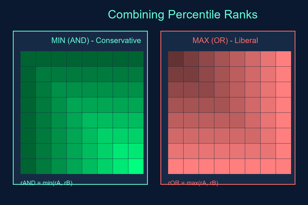
⚙️ Combining percentile ranks across features

If you have features A and B with ranks rA and rB:

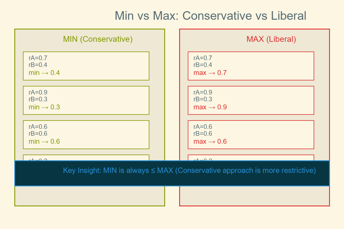
• 🔒 Conservative (AND-like) combination:

  rAND = min(rA, rB)

  → Combined score limited by the weaker (smaller) rank. Safe way to demand "both high."

• 🌈 Liberal (OR-like) combination:

  rOR = max(rA, rB)

  → Combined score benefits from the stronger (larger) rank. Allows "either high."

These match Day 1's logic mapping:

🧩 AND ≈ min OR ≈ max

They're simple, monotone, and explainable ✅

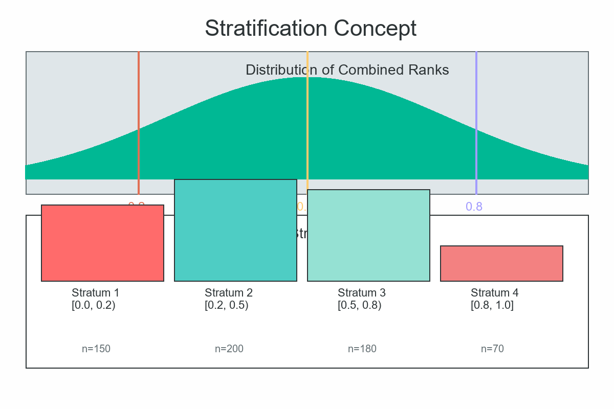
🧭 Stratification from Combined Ranks

Once you have a single combined rank per observation (e.g., rAND), split the population into strata:

• 🔢 Deciles: [0.0, 0.1, 0.2, …, 0.9, 1.0]

• 🧮 Quartiles: [0.0, 0.25, 0.5, 0.75, 1.0]

• ⚖️ Custom cuts: e.g., [0.0, 0.2, 0.5, 0.8, 1.0]

Use strata to:

• 🎯 Draw balanced samples

• 🚦 Prioritize reviews/interventions

• 📊 Report performance metrics by difficulty bands

Because ranks are monotone-invariant, your strata stay meaningful even if raw features change scale.

🧩 Solved example — From raw features to strata

Step 1️⃣: Compute percentile ranks per feature

Use the empirical CDF (rank = i/n). Example (rounded):

Step 2️⃣: Combine with min (AND-like) and max (OR-like)

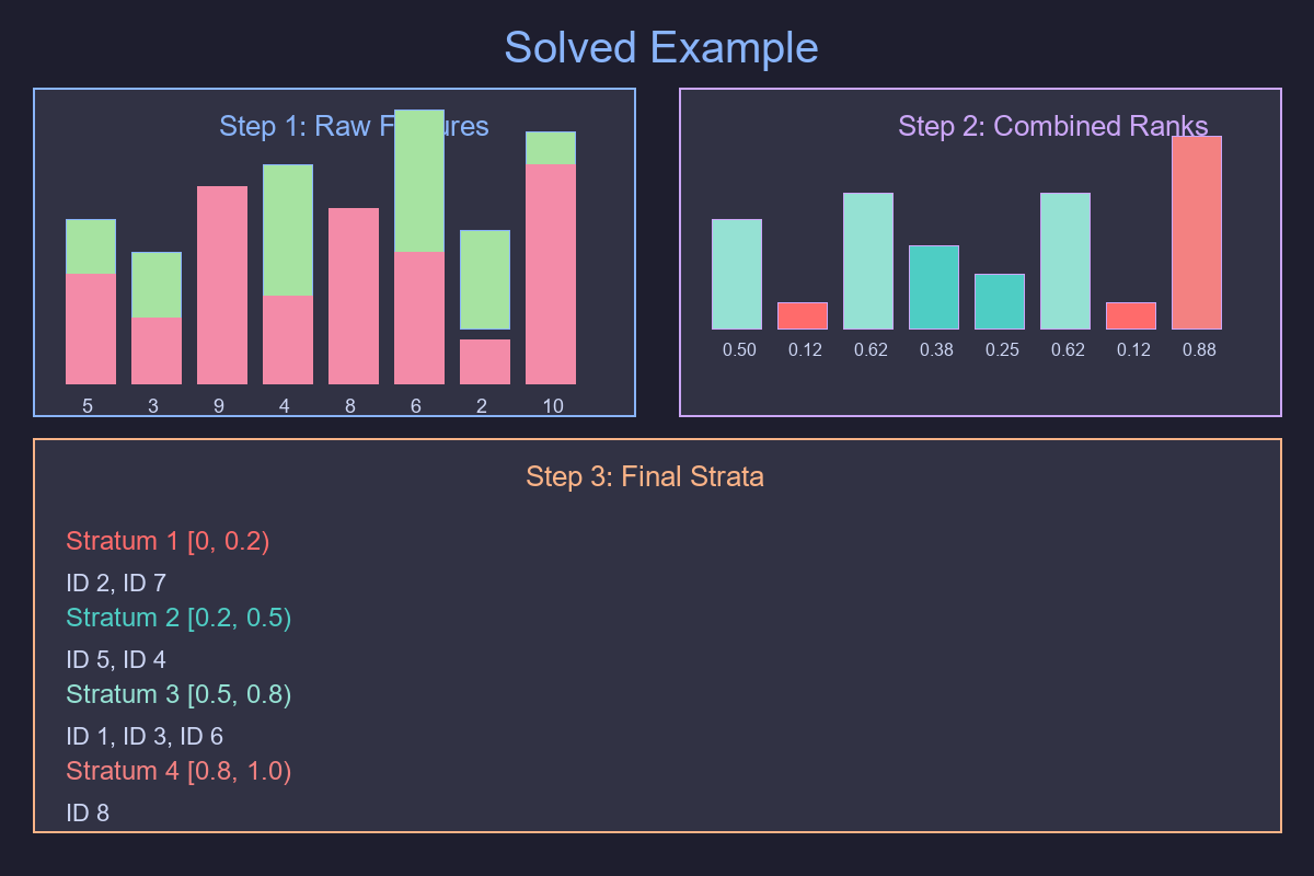
Step 3️⃣: Create strata from rAND

Cuts at 0.2, 0.5, 0.8 →

• 🩵 Stratum 1: rAND < 0.2 → ids 2, 7

• 💙 Stratum 2: 0.2 ≤ rAND < 0.5 → ids 5, 4

• 💜 Stratum 3: 0.5 ≤ rAND < 0.8 → ids 1, 3, 6

• 💛 Stratum 4: rAND ≥ 0.8 → id 8

📈 Using min is conservative: an observation only scores high if both A and B are high.

Using max is liberal — more points rise into higher strata.

💭 Why "min of ranks" is conservative

• rAND = min(rA, rB) can never exceed either input.

• Raising any rank can only lift (not drop) rAND.

• Thus, demanding high rAND ≈ saying "both inputs are high." ✅

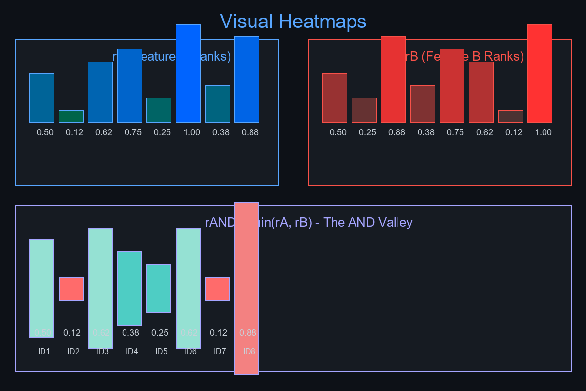
🖼️ Visual ideas

• 🧊 Two 2-D heatmaps:

  1️⃣ rA (x-axis = id, y-axis = rank) and rB similarly.

  2️⃣ The combined min(rA,rB) mesh — shows the "AND valley."

• 📊 Simple bar chart: rAND per id colored by stratum.

🧠 Practical tips

• 📦 Compute ranks per group for fair comparison (region/time).

• 🧾 Handle ties consistently (average ranks).

• 🪜 Pre-decide strata cuts (deciles, quartiles, custom).

• 🔄 Extend beyond two features:

  • rAND = min(r₁,…,rₖ)

  • rOR = max(r₁,…,rₖ)

🌟 Takeaway

Percentile ranks normalize features onto a common [0,1] scale.

Combining them with min (AND) or max (OR) gives an interpretable, monotone score ideal for sampling, prioritization, and reporting.

Simple ✅ Robust 🧩 Explainable 💡

📚 References

1. Hyndman, R. J., & Fan, Y. (1996). Sample quantiles in statistical packages. The American Statistician, 50(4), 361-365.

2. Serfling, R. J. (2009). Approximation Theorems of Mathematical Statistics. John Wiley & Sons.

3. Mosteller, F., & Tukey, J. W. (1977). Data Analysis and Regression: A Second Course in Statistics. Addison-Wesley.

4. Hoaglin, D. C., Mosteller, F., & Tukey, J. W. (Eds.). (1983). Understanding Robust and Exploratory Data Analysis. John Wiley & Sons.

5. David, H. A., & Nagaraja, H. N. (2003). Order Statistics (3rd ed.). John Wiley & Sons.

6. Parzen, E. (1979). Nonparametric statistical data modeling. Journal of the American Statistical Association, 74(365), 105-121.

7. Koenker, R. (2005). Quantile Regression. Cambridge University Press.

8. Langford, E. (2006). Quartiles in elementary statistics. Journal of Statistics Education, 14(3).

9. Hyndman, R. J. (1996). Computing and graphing highest density regions. The American Statistician, 50(2), 120-126.

10. Cramér, H. (1946). Mathematical Methods of Statistics. Princeton University Press.