Day 30: A Mathematical Blueprint for Robust Decision Frameworks
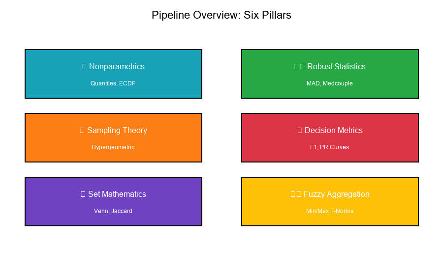
The Big Picture: Pipeline Overview
The decision framework pipeline transforms raw data into calibrated rules through six mathematical pillars:
Show code (11 lines)
ROBUST DECISION FRAMEWORK

Nonparametrics      Quantiles, ECDF, Order Statistics
Robust Statistics   MAD, Medcouple, Fences
Sampling Theory     Hypergeometric, Stratification
Decision Metrics    F1, Precision, Recall, PR Curves
Set Mathematics     Venn Diagrams, Jaccard Index
Fuzzy Aggregation   Min/Max T-Norms, Rule Combination
Visual Example:
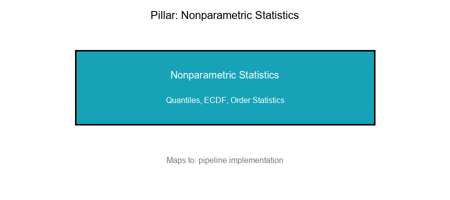
Pillar 1: Nonparametric Statistics
Key Concepts
Quantiles and Percentiles:
- No distributional assumptions
- Data-driven thresholds
- Robust to outliers
ECDF (Empirical CDF):
F̂_n(x) = (1/n) × |{i : X_i ≤ x}|
Order Statistics:
X_(1) ≤ X_(2) ≤ ... ≤ X_(n)
Pipeline Mapping
| Concept | Implementation | Purpose |
|---------|---------------|---------|
| Quantiles | np.percentile() | Threshold computation |
| ECDF | statsmodels.ECDF() | Distribution visualization |
| Order stats | np.sort() | Ranking, outlier detection |
Code-Math Connection
# Mathematical: Q(p) = F⁻¹(p)
# Code implementation:
threshold = np.percentile(data, 90)  # 90th percentile

# Mathematical: F̂_n(x) = (1/n)Σ{X_i ≤ x}
# Code implementation:
ecdf = lambda x: np.mean(data <= x)
Visual Example:
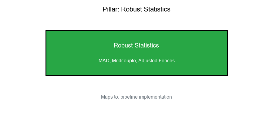
Pillar 2: Robust Statistics
Key Concepts
MAD (Median Absolute Deviation):
MAD = median(|X_i - median(X)|)
Medcouple (Asymmetry Measure):
MC = median{ h(x_i, x_j) : x_i ≤ median ≤ x_j }
Adjusted Boxplot Fences:
Lower: Q1 - 1.5 × IQR × e^(-4MC)  if MC ≥ 0
Upper: Q3 + 1.5 × IQR × e^(3MC)   if MC ≥ 0
Pipeline Mapping
| Concept | Implementation | Purpose |
|---------|---------------|---------|
| MAD | Custom or scipy.stats.median_abs_deviation | Robust scale |
| Medcouple | Custom implementation | Skewness detection |
| Fences | Adjusted boxplot formulas | Outlier boundaries |
Code-Math Connection
Show code (10 lines)
# Mathematical: MAD = median(|X - median(X)|)
# Code implementation:
def mad(data):
median_val = np.median(data)
return np.median(np.abs(data - median_val))

# Mathematical: σ_robust ≈ 1.4826 × MAD
# Code implementation:
robust_std = 1.4826 * mad(data)
Visual Example:
Pillar 3: Sampling Theory
Key Concepts
Hypergeometric Distribution:
P(X = k) = C(K,k) × C(N-K, n-k) / C(N, n)
Stratified Sampling:
n_h = n × (N_h / N)  [Proportional]
n_h = n × (N_h × σ_h) / Σ(N_j × σ_j)  [Neyman]
Power Analysis:
n = ((z_α + z_β)² × σ²) / δ²
Pipeline Mapping
| Concept | Implementation | Purpose |
|---------|---------------|---------|
| Hypergeometric | scipy.stats.hypergeom | Exact probabilities |
| Stratification | Custom allocation | Sample optimization |
| Power | Sample size formulas | Study design |
Code-Math Connection
Show code (11 lines)
# Mathematical: P(X = k) from hypergeometric
# Code implementation:
from scipy.stats import hypergeom
prob = hypergeom.pmf(k=5, M=100, n=20, N=30)

# Mathematical: Neyman allocation
# Code implementation:
def neyman_allocation(N_h, sigma_h, n_total):
weights = N_h * sigma_h
return n_total * weights / weights.sum()
Visual Example:
Pillar 4: Decision Metrics
Key Concepts
Precision and Recall:
Precision = TP / (TP + FP)
Recall = TP / (TP + FN)
F1 Score:
F1 = 2 × (Precision × Recall) / (Precision + Recall)
PR Curve:
{(Recall(τ), Precision(τ)) : τ ∈ [0, 1]}
Pipeline Mapping
| Concept | Implementation | Purpose |
|---------|---------------|---------|
| Confusion matrix | sklearn.metrics.confusion_matrix | Classification summary |
| F1 Score | sklearn.metrics.f1_score | Balanced metric |
| PR Curve | sklearn.metrics.precision_recall_curve | Threshold selection |
Code-Math Connection
Show code (11 lines)
# Mathematical: F1 = 2PR / (P + R)
# Code implementation:
from sklearn.metrics import f1_score
f1 = f1_score(y_true, y_pred)

# Mathematical: Find τ* = argmax F1(τ)
# Code implementation:
precisions, recalls, thresholds = precision_recall_curve(y_true, scores)
f1_scores = 2 * precisions * recalls / (precisions + recalls + 1e-10)
optimal_threshold = thresholds[np.argmax(f1_scores)]
Visual Example:
Pillar 5: Set Mathematics
Key Concepts
Set Operations:
Intersection: A ∩ B = {x : x ∈ A and x ∈ B}
Union: A ∪ B = {x : x ∈ A or x ∈ B}
Jaccard Index:
J(A, B) = |A ∩ B| / |A ∪ B|
Inclusion-Exclusion:
|A ∪ B| = |A| + |B| - |A ∩ B|
Pipeline Mapping
| Concept | Implementation | Purpose |
|---------|---------------|---------|
| Intersection | set.intersection() | Overlap analysis |
| Jaccard | Custom formula | Similarity measurement |
| Venn diagrams | matplotlib_venn | Visualization |
Code-Math Connection
Show code (11 lines)
# Mathematical: J(A, B) = |A ∩ B| / |A ∪ B|
# Code implementation:
def jaccard_index(set_a, set_b):
intersection = len(set_a & set_b)
union = len(set_a | set_b)
return intersection / union if union > 0 else 0

# Mathematical: |A ∪ B| = |A| + |B| - |A ∩ B|
# Code implementation:
union_size = len(set_a) + len(set_b) - len(set_a & set_b)
Visual Example:
Pillar 6: Fuzzy Aggregation
Key Concepts
T-Norms (AND):
Minimum: T_min(x, y) = min(x, y)
Product: T_prod(x, y) = x × y
Łukasiewicz: T_Luk(x, y) = max(0, x + y - 1)
T-Conorms (OR):
Maximum: S_max(x, y) = max(x, y)
Idempotence:
min(x, x) = x
x × x = x²
Pipeline Mapping
| Concept | Implementation | Purpose |
|---------|---------------|---------|
| Min/Max | np.minimum, np.maximum | Rule aggregation |
| T-norms | Custom functions | Fuzzy AND |
| Idempotence | Property of min | Stable aggregation |
Code-Math Connection
Show code (13 lines)
# Mathematical: AND via min (idempotent)
# Code implementation:
def fuzzy_and(values):
return np.min(values)

# Mathematical: OR via max
# Code implementation:
def fuzzy_or(values):
return np.max(values)

# Rule evaluation
rule_strength = fuzzy_and([condition1, condition2, condition3])
Visual Example:
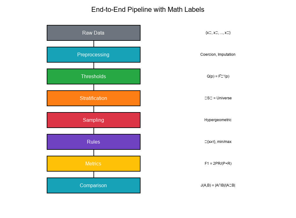
End-to-End Diagram with Math Labels
The Complete Pipeline
Show code (40 lines)
RAW DATA
{x₁, x₂, ..., xₙ}
PREPROCESSING
• Coercion: string → numeric
• Imputation: NA → 0 or median
• Impact: Shifts F̂(x), quantiles
THRESHOLD COMPUTATION
• Quantiles: Q(p) = F̂⁻¹(p)
• MAD fences: Q₂ ± k × MAD
• Adjusted bounds: exp(±f(MC))
STRATIFICATION
• Partition: ∪ Sₕ = Universe, Sₕ ∩ S = ∅
• Risk levels: π₁(h) = P(Fraud|h)
• Cost weights: C₁₀(h), C₀₁(h)
SAMPLING
• Hypergeometric: P(X=k) = C(K,k)C(N-K,n-k)/C(N,n)
• Power: n = ((z_α+z_β)²σ²)/δ²
• Allocation: Proportional, Neyman, Risk-weighted
RULE EVALUATION
• Indicator functions: {x ≥ τ}
• Fuzzy AND: min(c₁, c₂, ..., cₖ)
• Fuzzy OR: max(c₁, c₂, ..., cₖ)
DECISION METRICS
• Precision: TP/(TP+FP)
• Recall: TP/(TP+FN)
• F1: 2PR/(P+R)
COMPARISON & ADJUSTMENT
• Set overlap: J(A,B) = |A∩B|/|A∪B|
• Threshold adjustment: τ* = C₀₁/(C₀₁+C₁₀)
• Feedback loop: Update priors, costs
Visual Example:
Exercise: Write a Methodology Abstract
The Problem
Write a short methodology abstract (150-200 words) that references each mathematical building block.
Solution
Methodology Abstract
This robust decision framework employs a mathematically rigorous approach to threshold-based decision making. We begin with nonparametric quantile estimation using empirical cumulative distribution functions (ECDF) and order statistics to establish data-driven thresholds without distributional assumptions.
To handle skewed and outlier-prone data, we apply robust statistics including the Median Absolute Deviation (MAD) and medcouple-adjusted boxplot fences that adapt to asymmetric distributions.
Stratified sampling with hypergeometric probability models ensures representative coverage across risk segments, with sample sizes determined by power analysis to detect meaningful deviations.
Rule conditions are combined using fuzzy logic operators (min/max t-norms) that provide idempotent, conservative aggregation. Performance is evaluated through decision metrics including precision, recall, and F1 score, with Precision-Recall curves guiding threshold optimization.
Finally, set-theoretic analysis via Jaccard indices and Venn diagrams quantifies overlap between rule versions, enabling systematic comparison and refinement. This integrated mathematical framework ensures calibrated, defensible, and continuously improvable decision rules.
Word count: 175 words
Mini-Glossary
| Term | Definition |
|---|---|
| ECDF | Empirical Cumulative Distribution Function: F̂(x) = proportion ≤ x |
| Order Statistics | Sorted sample values: X₍₁₎ ≤ X₍₂₎ ≤ ... ≤ X₍ₙ₎ |
| Medcouple | Robust measure of skewness, range [-1, 1] |
| Hypergeometric | Distribution for sampling without replacement |
| T-Norm | Fuzzy AND operator satisfying specific axioms |
| Idempotence | Property: T(x, x) = x (only min satisfies this) |
30-Day Journey Summary
Week 1: Foundations (Days 1-7)
- Data distributions and visualization
- Basic statistics and summaries
- Introduction to thresholds
Week 2: Quantiles & Robustness (Days 8-14)
- Percentiles and ECDF
- MAD and robust measures
- Medcouple and adjusted fences
Week 3: Sampling & Decisions (Days 15-21)
- Hypergeometric distribution
- Stratified sampling
- Power analysis
- Decision metrics
Week 4: Logic & Integration (Days 22-28)
- Set theory and Venn diagrams
- ATL/BTL partitioning
- Cost-sensitive thresholds
- Fuzzy logic aggregation
Week 5: Synthesis (Days 29-30)
- Complete audit plan
- Mathematical blueprint
Final Thoughts
After 30 days, you now have a complete mathematical toolkit for building robust decision frameworks:
The Six Pillars:
- Nonparametrics: Data-driven, assumption-free thresholds
- Robust Statistics: Outlier-resistant measures
- Sampling Theory: Efficient, valid inference
- Decision Metrics: Performance measurement
- Set Mathematics: Comparison and overlap
- Fuzzy Aggregation: Rule combination
The Journey:
- From raw data to calibrated decisions
- From intuition to mathematical rigor
- From ad-hoc to systematic
Key Takeaways:
Quantiles provide distribution-free thresholds MAD and medcouple resist outliers and skewness Hypergeometric models exact sampling probabilities F1 score balances precision and recall Jaccard index measures set similarity Min/max provides idempotent rule aggregation
You now have the mathematical blueprint. Go build robust scenarios!
Congratulations!
You've completed the 30-Day Mathematical Foundations for Robust Decision Frameworks series!
What you've learned:
- Rigorous mathematical foundations
- Practical implementation patterns
- Code-agnostic understanding
- End-to-end pipeline thinking
Next steps:
- Apply these concepts to your own data
- Experiment with different parameter choices
- Build and refine your calibration workflows
- Share your learnings with your team
Thank you for joining this journey!