Day 9 — Z-Scores vs Robust Z-Scores ⚔️📊

When one wild point can topple the mean, it is time to switch to statistics that fight back.

💡 Note: This article uses technical terms and abbreviations. For definitions, check out the Key Terms & Glossary page.

🎯 Introduction

The classical z-score normalizes data by subtracting the mean and dividing by the standard deviation. It shines when data are clean and approximately normal. Yet a single wild observation can warp both statistics, hiding true outliers the moment you need detection most.

TL;DR:

• Classical z-scores depend on the mean and standard deviation, both of which have a 0% breakdown point and an unbounded influence function.
• Robust z-scores swap in the median and MAD (Median Absolute Deviation) so half the data must be corrupted before things collapse.
• Use classical z-scores for clean, well-behaved measurements; prefer robust z-scores as your default for messy, real-world datasets.

💕➡️💔 The Classic Z-Score: Powerful Until It Isn't

The z-score answers a timeless question: “How many standard deviations away from the mean is this point?”

z = (x - μ) / σ

Where x is the data value, μ is the sample mean, and σ is the sample standard deviation. Analysts flag |z| > 3 (sometimes 2.5) as suspicious.

With clean values like [10, 12, 11, 13, 12, 14, 11, 13, 12, 11], it works brilliantly:

μ = 11.9
σ = 1.2
z(20) = (20 - 11.9) / 1.2 = 6.75  ✅ obvious outlier

Add a single rogue point and everything crumbles:

Contaminated data: [10, 12, 11, 13, 12, 14, 11, 13, 12, 1000]
μ = 110.8
σ = 295.7
z(20) = (20 - 110.8) / 295.7 = -0.31 ❌ hidden
z(1000) = (1000 - 110.8) / 295.7 = 3.01  😬 barely flagged

The outlier throws off the very yardsticks being used to detect it.

💣 Breakdown Points & Influence: Why Collapse Happens

The breakdown point measures how much contamination a statistic can tolerate. The mean and standard deviation have a 0% breakdown point—one extreme value can drive them to infinity. Their influence functions are unbounded, meaning the further a point is from the center, the more it drags the statistic along.

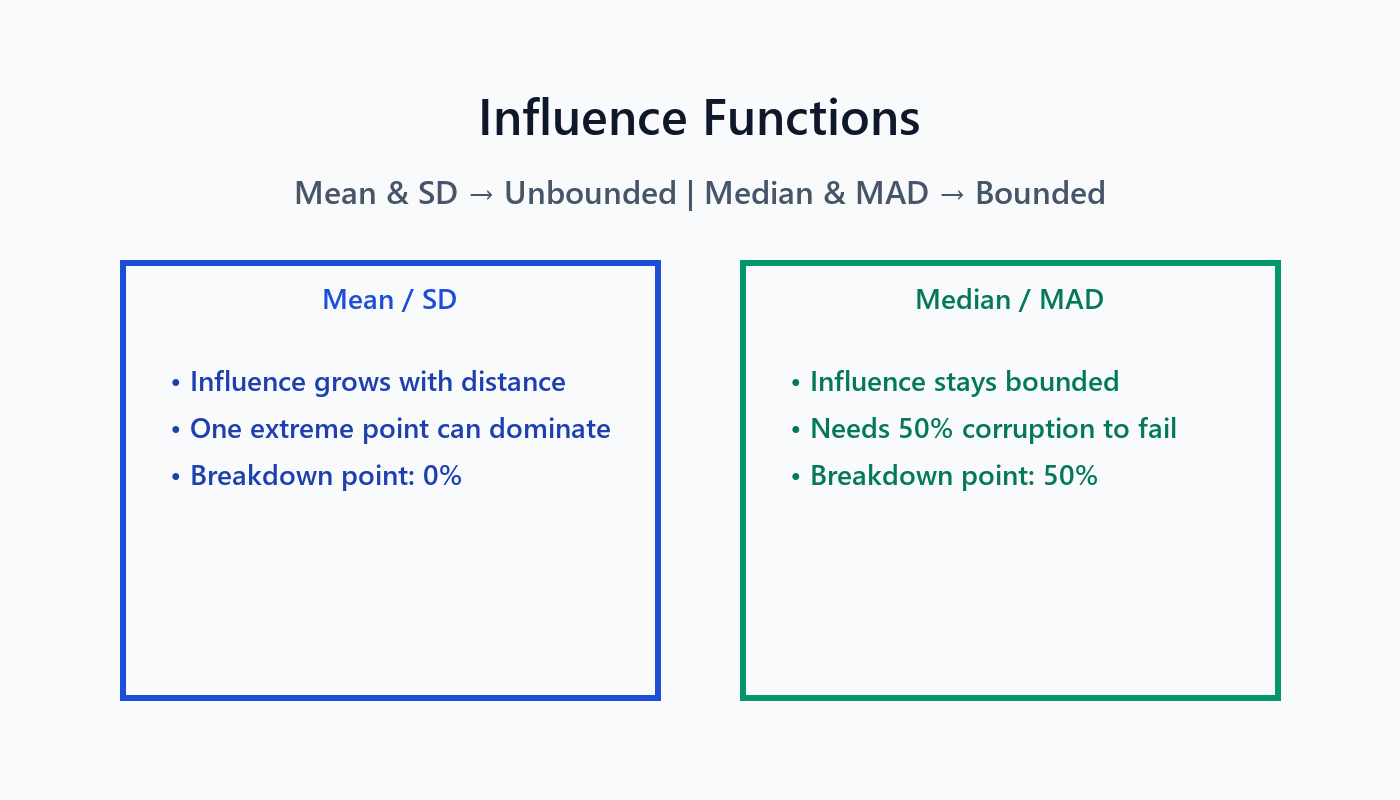
By contrast, the median and MAD boast a 50% breakdown point and bounded influence. Half the sample must be corrupted before they crumble.

🛡️ Median & MAD: The Robust Duo

The median is the middle value of sorted data. It takes a concerted attack on at least half the sample to move it.

The MAD (Median Absolute Deviation) measures spread without trusting the mean:

MAD = median(|xᵢ - median(x)|)
MAD* = 1.4826 × MAD

The constant 1.4826 rescales MAD so that MAD* ≈ σ for normally distributed samples. Together, the median and MAD supply a resilient center and scale for the same z-score formula.

🧮 Classical vs Robust Formulas

| Step | Classical z-score | Robust z-score | |------|-------------------|----------------| | Center | μ = (1/n) Σ xᵢ | median(x) | | Spread | σ = √[(1/n) Σ (xᵢ − μ)²] | MAD* = 1.4826 × median(|xᵢ − median(x)|) | | Score | zᵢ = (xᵢ − μ) / σ | zᵢᵣ = (xᵢ − median) / MAD* | | Typical threshold | |zᵢ| > 3 | |zᵢᵣ| > 3.5 |

Classical statistics are optimal for pristine Gaussian data; robust statistics remain useful when normality is a pipe dream.

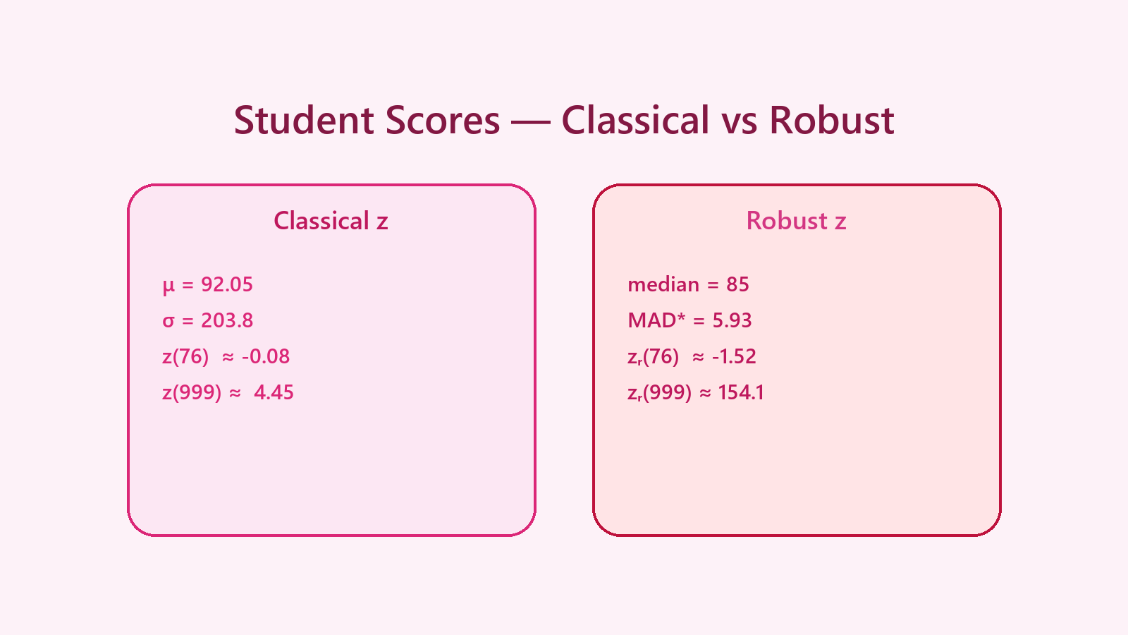
🔬 Walkthrough: Student Scores Gone Wrong

Dataset with a fat-fingered entry:

[78, 82, 85, 79, 91, 88, 76, 84, 89, 87,
 83, 80, 86, 92, 81, 85, 999, 88, 84, 90]

Classical z-score:

μ = 92.05
σ ≈ 203.8
z(76)  ≈ -0.08  → “perfectly normal”
z(999) ≈  4.45  → barely past the 3σ rule

Robust z-score:

median = 85
MAD = 4
MAD* = 5.93
zᵣ(76)  = (76 - 85) / 5.93  ≈ -1.52
zᵣ(999) = (999 - 85) / 5.93 ≈ 154.1 🚨

The robust approach instantly isolates the malformed record while keeping authentic scores unflagged.

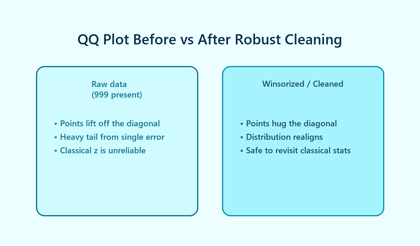
📈 Visual Diagnostics Matter

Quantile-Quantile (QQ) plots reveal how a single outlier bends the distribution away from normality. Before winsorizing or trimming, the top-right point rockets off the diagonal. After robust cleaning, the plot settles back onto the line, signaling that classical techniques may again be appropriate.

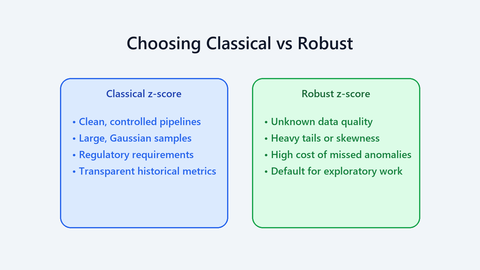
🧭 Choosing the Right Tool

Favour classical z-scores when:

• Instrumentation enforces quality and the dataset is demonstrably clean.
• You are confirming findings with large, well-behaved samples.
• Industry regulations require the traditional formula.

Favour robust z-scores when:

• Data provenance is unknown or messy (the default in the wild).
• Sample sizes are modest and every point counts.
• Skewed, heavy-tailed, or multi-modal distributions appear in diagnostics.
• Missing a real anomaly would be catastrophic.

🛠️ Code Snippets

import numpy as np

def zscore_outliers(data, threshold=3.0):
    mean = np.mean(data)
    std = np.std(data)
    scores = (data - mean) / std
    return data[np.abs(scores) > threshold]

def robust_zscore_outliers(data, threshold=3.5):
    median = np.median(data)
    mad = np.median(np.abs(data - median))
    mad_star = 1.4826 * mad
    scores = (data - median) / mad_star
    return data[np.abs(scores) > threshold]

Run both; large disagreements are an immediate red flag that classical assumptions failed.

🌟 Takeaway

• Classical z-scores crumble in the face of even one contaminated point.
• Robust z-scores powered by the median and MAD withstand up to 50% corruption.
• Use diagnostics, iterate, and document which yardstick you chose (and why).

🔭 Coming Up Next

Day 10 dives into Local Outlier Factor (LOF) to catch anomalies hiding in low-density pockets of high-dimensional space. 🔍

📚 References

• Rousseeuw, P.J., & Croux, C. (1993). Alternatives to the Median Absolute Deviation. Journal of the American Statistical Association.
• Hampel, F.R. (1974). The Influence Curve and Its Role in Robust Estimation. Journal of the American Statistical Association.
• Wilcox, R.R. (2017). Introduction to Robust Estimation and Hypothesis Testing.

✨ Thanks for geeking out with me on robust statistics—see you tomorrow! ✨