Day 6 — Distribution Shape: Skewness and Kurtosis (Simple Guide + Visuals)
*Understanding distribution shape! *
Introduction
While mean and variance tell us about the center and spread of data, skewness and kurtosis reveal the shape of the distribution. Understanding these shape features helps us choose appropriate methods for outlier detection, binning, and modeling.
In a nutshell:
Skewness tells you if data lean left or right (asymmetry). ↩↪
Kurtosis tells you how heavy the tails are (how many extremes you see).
Two datasets can share the same mean and variance but look completely different — shape features reveal the hidden story.
Knowing shape helps you choose better outlier rules, bins, and models.
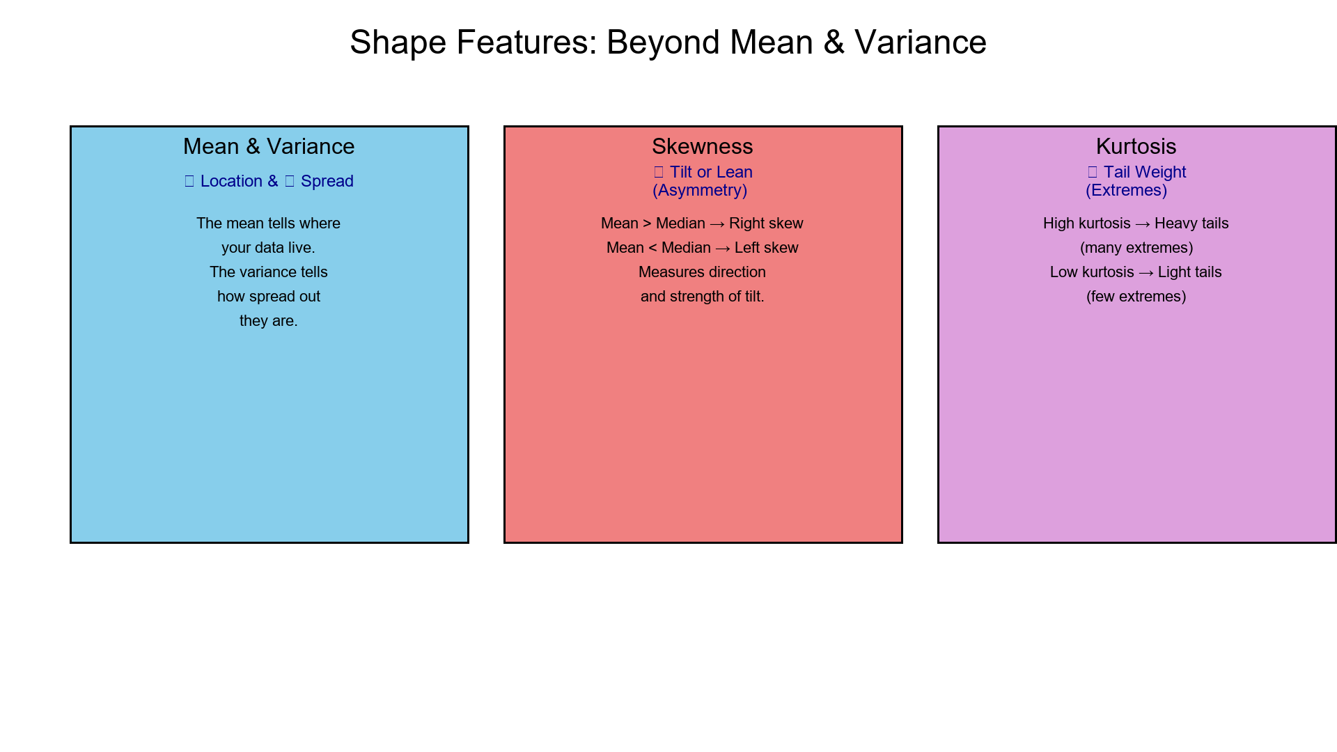
1. What "shape features" mean
The mean says where your data live.
The variance says how spread out they are.
But the shape — captured by skewness and kurtosis — says what personality your data have.
Think of:
Skewness = tilt or lean
Kurtosis = tail weight (heaviness of extremes)
Same center + same spread ≠ same shape.
One can be tall and thin, another flat and wide, another lopsided — and each tells a different story.
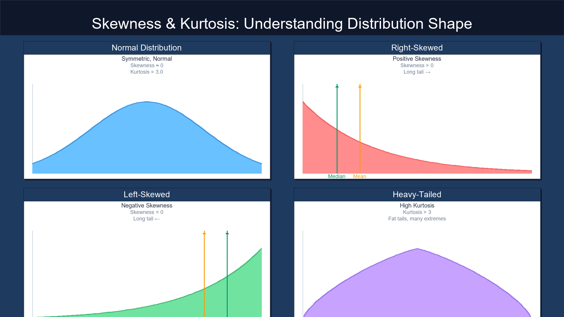
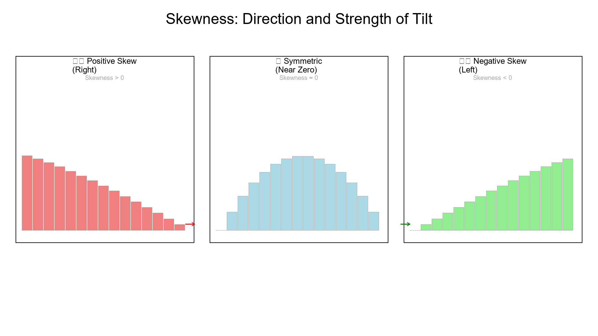
2. Skewness = Asymmetry ↩↪
Positive skew (right-skewed): long tail to the right — a few large values pull the distribution.
Negative skew (left-skewed): long tail to the left — a few small values drag it down.
Near zero skew: roughly symmetric.
Quick mental check:
- Mean > Median → Right skew
- Mean < Median → Left skew
How it's computed (idea):
Skewness measures the average signed distance of points from the mean, scaled by their spread.
You don't need to calculate it manually — just know it quantifies tilt.
Where it matters:
- Amounts, durations, and counts are often right-skewed.
- Strong skew breaks "normality" assumptions and messes with classical z-scores.
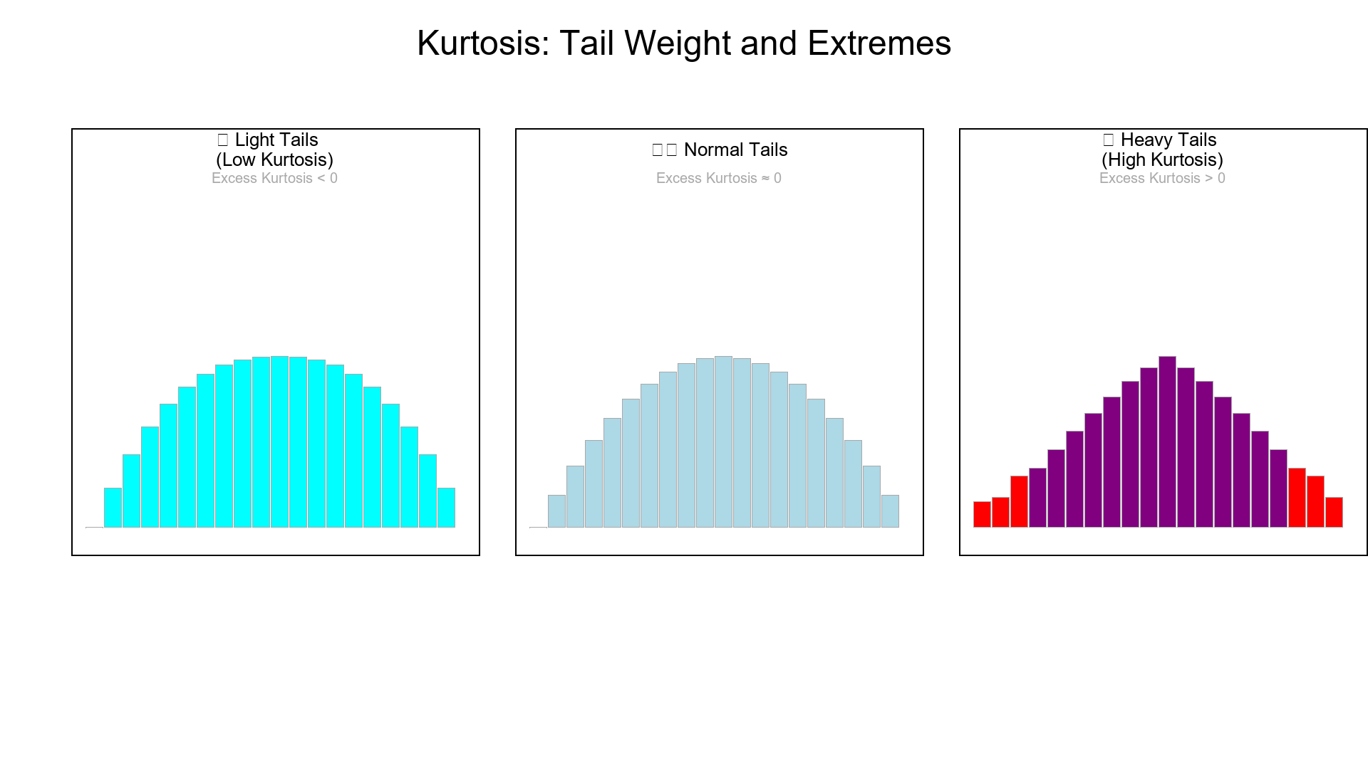
3. Kurtosis = Tail Weight
High kurtosis (leptokurtic): heavy tails → many extremes.
Low kurtosis (platykurtic): light tails → few extremes.
Normal distribution has kurtosis = 3.
"Excess kurtosis" = kurtosis − 3 → Normal ⇒ 0 excess.
Myth alert: Kurtosis is about tails, not peakedness.
You can have a tall center and still light tails —or a flat center with heavy tails.
Practical impact:
- Heavy tails → Mean/SD get distorted; use Median/MAD and robust z-scores.
- Light tails → Classic mean/SD methods behave predictably.
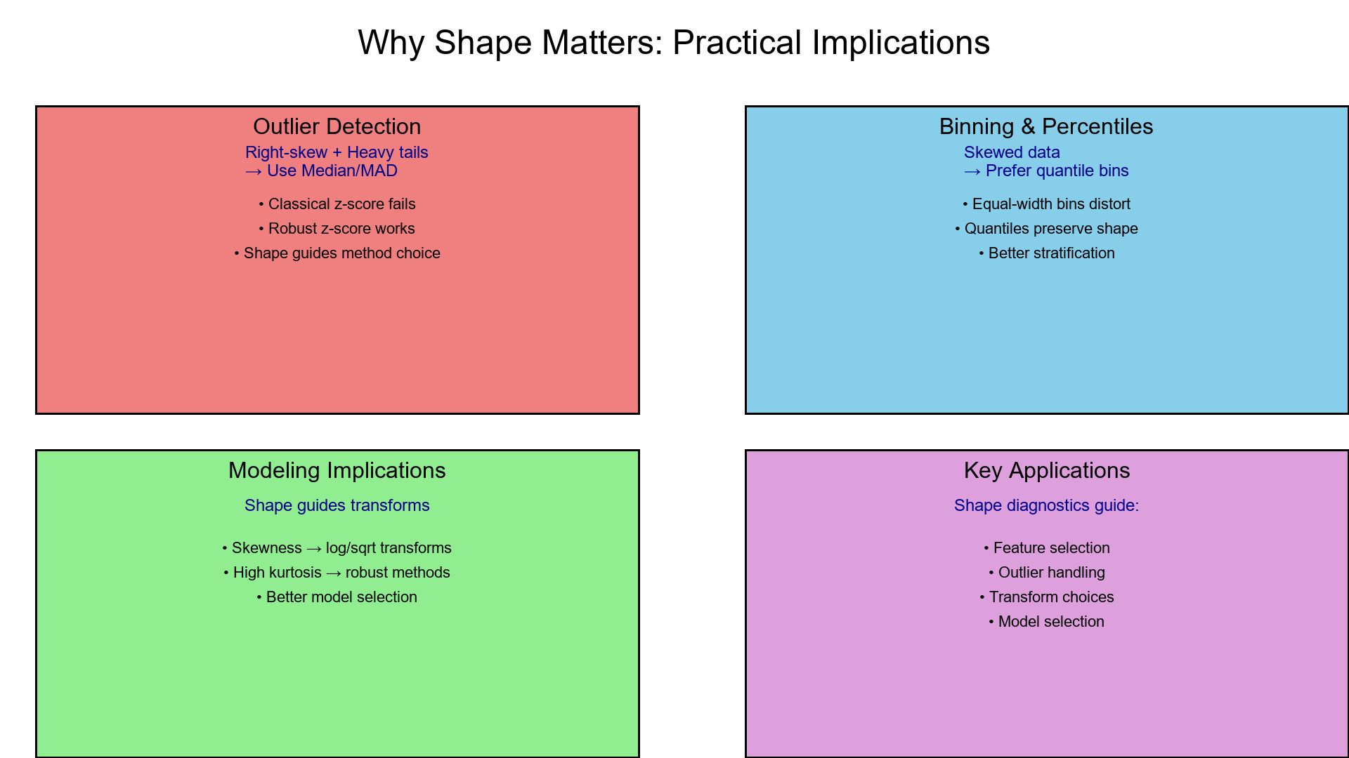
4. Why You Should Care
Outlier Detection:
- Right-skew + heavy tails → use robust stats (Median/MAD).
- Symmetric + light tails → classical z-score is fine.
Binning and Percentiles:
- Skewed data → prefer quantile bins over equal-width.
Modeling Implications:
- Skewness → consider log/sqrt transforms for variance stability.
- High kurtosis → expect many extremes → try quantile loss or robust regressions.
Use shape diagnostics like get_skewness_kurtosis() to guide cleaning, binning, and feature selection.
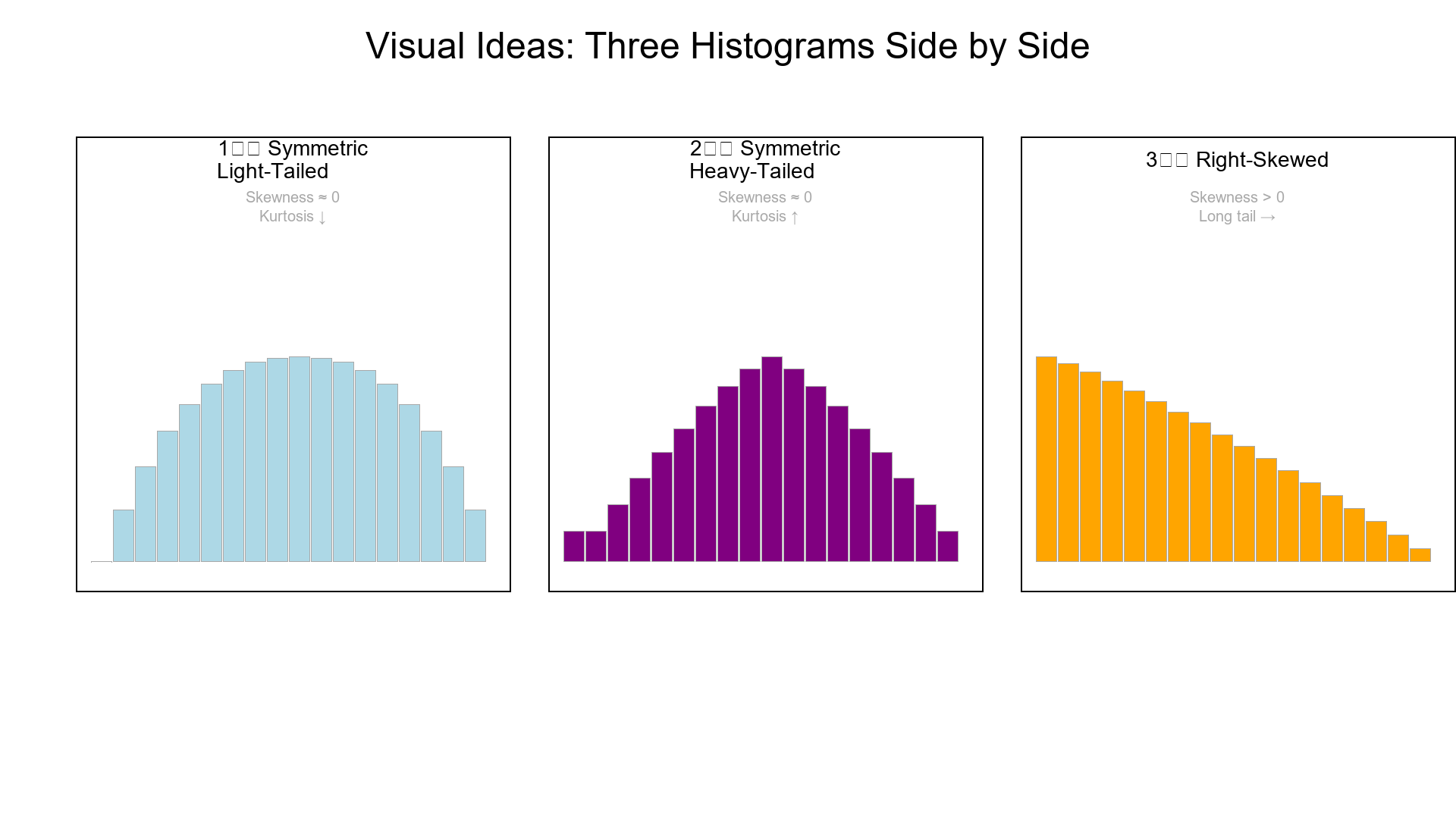
5. Three Shapes, Same Mean & Variance
Imagine three histograms with the same mean and variance:
| Shape | Skewness | Kurtosis | Description |
|---|---|---|---|
| Symmetric light-tailed | ≈ 0 | < 3 | Bell-shaped, few extremes |
| Symmetric heavy-tailed | ≈ 0 | > 3 | Frequent highs and lows |
| Right-skewed | > 0 | > 3 | Many small values, few big ones |
All have identical center and spread — but completely different risk and outlier profiles.

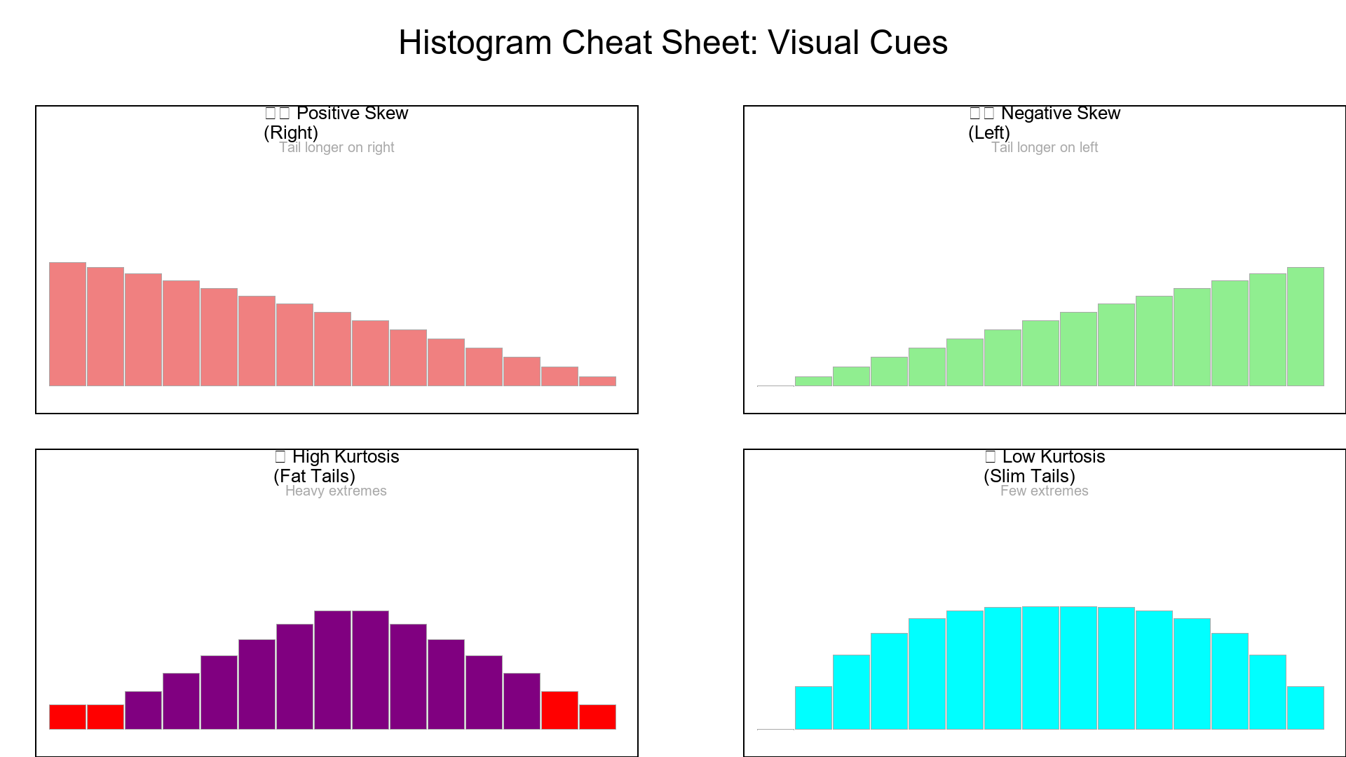
6. Histogram Cheat Sheet
- Tail longer on right → Positive skew
- Tail longer on left → Negative skew
- Fat tails → High kurtosis
- Slim tails → Low kurtosis
Visual cue = instant intuition.
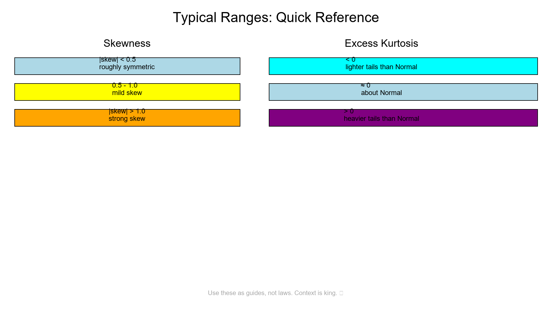
7. Typical Ranges (Quick Rules)
Skewness:
- |skew| < 0.5 → roughly symmetric
- 0.5–1 → mild skew
- |skew| > 1 → strong skew
Excess Kurtosis (kurtosis − 3):
- < 0 → lighter tails than Normal
- ≈ 0 → about Normal
-
0 → heavier tails than Normal
Use these as guides, not laws. Context is king.
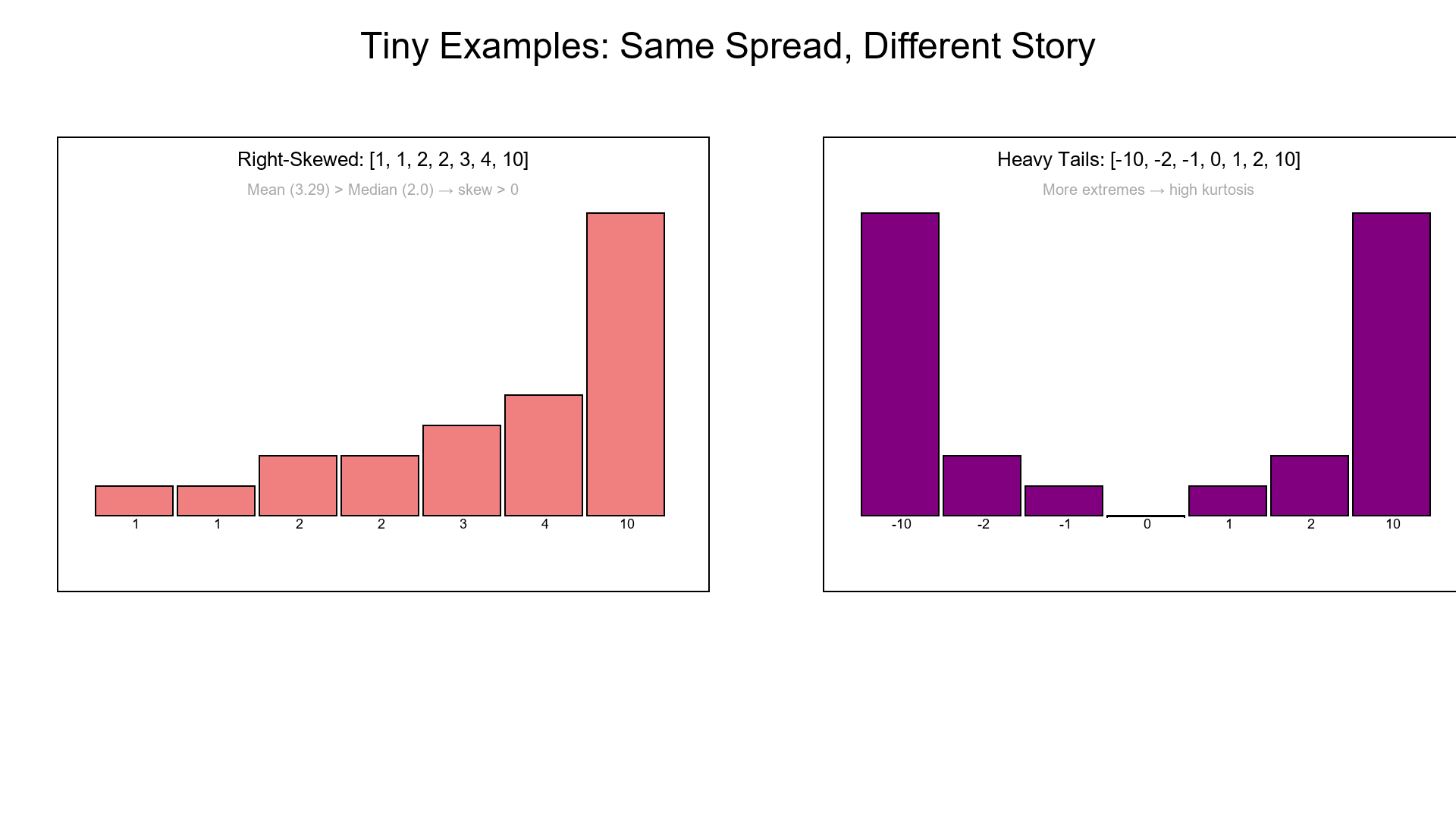
8. Tiny Examples
Right-skewed: [1, 1, 2, 2, 3, 4, 10] → mean > median → skew > 0.
Heavy tails: [−10, −2, −1, 0, 1, 2, 10] → more extremes → high kurtosis.
Same spread, different story.
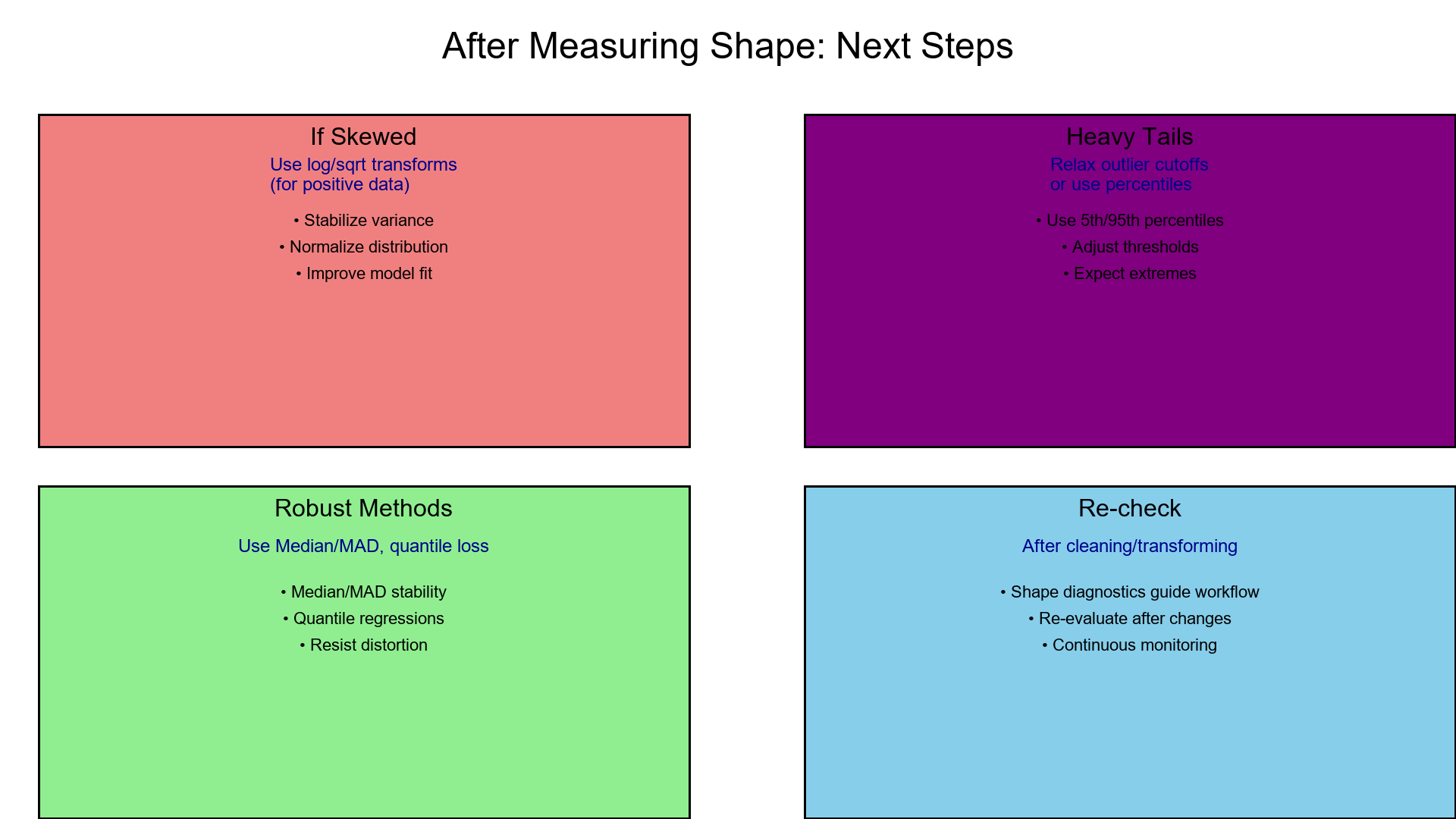
9. After Measuring Shape
- If skewed → use log/sqrt transforms (for positive data).
- For heavy tails → relax outlier cutoffs or use percentiles (5th/95th).
- Use robust methods (Median/MAD, quantile loss) for stability.
- Re-check skew/kurtosis after cleaning or transforming.
Visual Ideas
Show three histograms (side by side):
-
Symmetric light-tailed
-
Symmetric heavy-tailed
-
Right-skewed
Annotate each with "Skewness sign" and "Kurtosis ↑ / ↓".
⏱ One-Minute Summary
- Skewness = direction and strength of tilt.
- Kurtosis = tail heaviness (extremes).
- Mean & variance alone can mislead — shape completes the picture.
- Knowing shape → better thresholds, bins, transforms, and models.
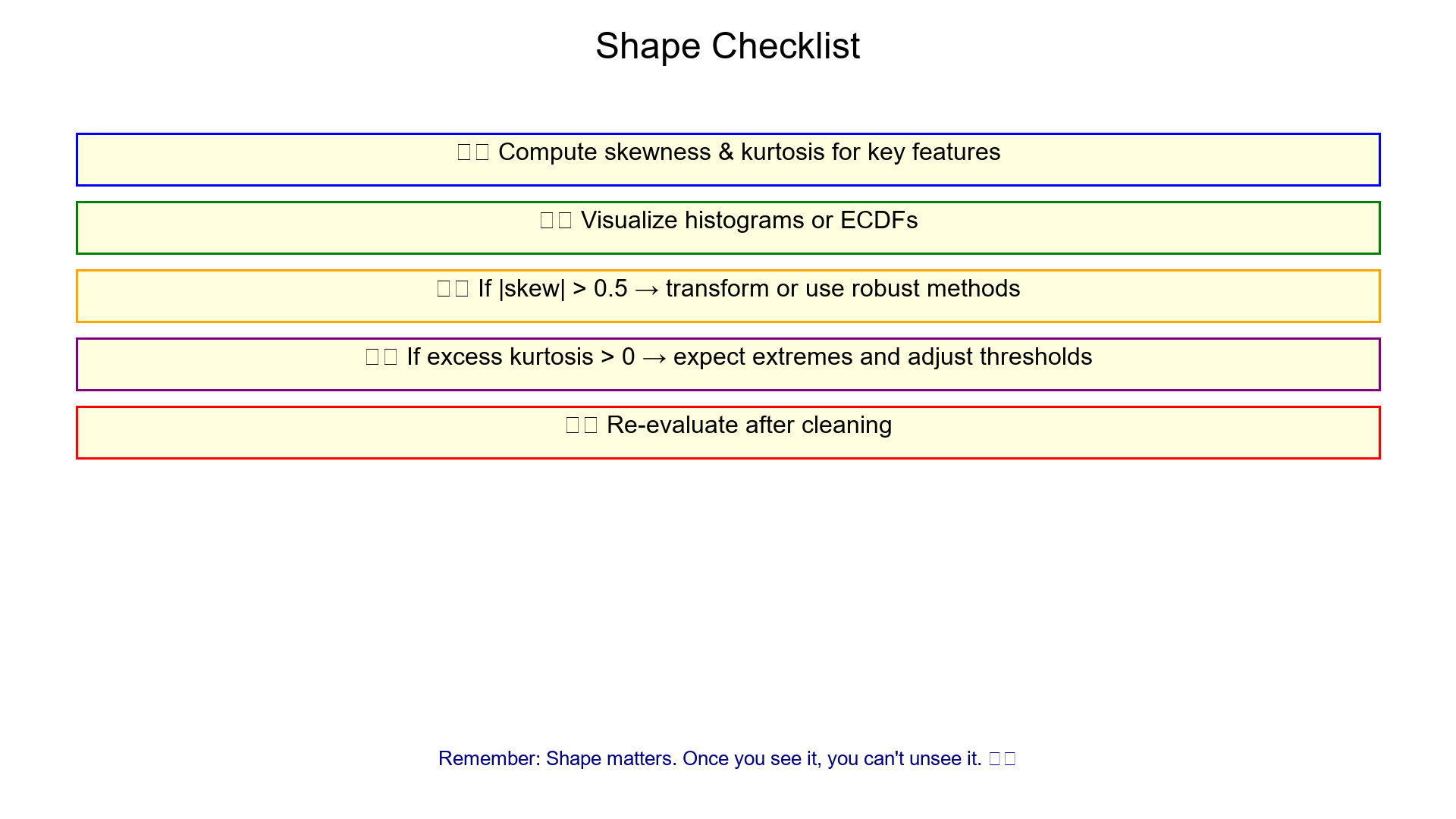
Shape Checklist
Compute skewness & kurtosis for key features
Visualize histograms or ECDFs
If |skew| > 0.5 → transform or use robust methods
If excess kurtosis > 0 → expect extremes and adjust thresholds
Re-evaluate after cleaning
Wrapping Up
Every dataset has a shape signature.
Skewness and kurtosis let you read it like a fingerprint — revealing tilt, tail, and trustworthiness.
They don't just decorate your summary table — they guide how you treat outliers, split bins, and choose models.
Shape matters.
And once you see it, you can't unsee it.
References
-
Joanes, D. N., & Gill, C. A. (1998). Comparing measures of sample skewness and kurtosis. Journal of the Royal Statistical Society: Series D (The Statistician), 47(1), 183-189.
-
DeCarlo, L. T. (1997). On the meaning and use of kurtosis. Psychological Methods, 2(3), 292-307.
-
Westfall, P. H. (2014). Kurtosis as peakedness, 1905–2014. R.I.P. The American Statistician, 68(3), 191-195.
-
Pearson, K. (1895). Contributions to the mathematical theory of evolution. II. Skew variation in homogeneous material. Philosophical Transactions of the Royal Society of London, 186, 343-414.
-
Fisher, R. A. (1930). The moments of the distribution for normal samples of measures of departure from normality. Proceedings of the Royal Society of London. Series A, 130(812), 16-28.
-
Tukey, J. W. (1977). Exploratory Data Analysis. Addison-Wesley.
-
Hoaglin, D. C., Mosteller, F., & Tukey, J. W. (Eds.). (1983). Understanding Robust and Exploratory Data Analysis. John Wiley & Sons.